|
|
|
|
Moveout-based wave-equation migration velocity analysis |
 sensitivity kernel calculation
operator.
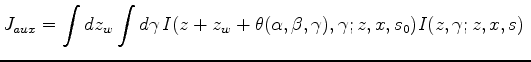
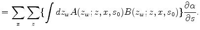
The approach is to define the auxilary function that links moveout parameter
sensitivity kernel calculation
operator.
The approach is to define the auxilary function that links moveout parameter
 and the slowness
Notice that here the moveout between the initial image
Since
![]() maximize eq (11),
maximize eq (11),
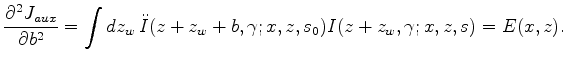
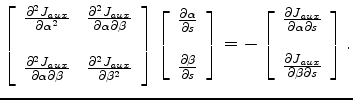
We differentiate the equation (12) with respect to
![]() and
and ![]() , which gives
, which gives
![$\displaystyle \left[ \begin{array}{cc} \frac{\partial^2{J_{aux}}}{\partial{\alp...
...\ \\ \frac{\partial{J_{aux}}}{\partial{\beta}\partial{s}} \end{array} \right] .$](img102.png) |
(13) |
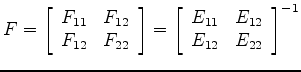
Now we need to invert a Jacobian to get
 . We define the following:
Then
 |
(15) |
There is another way to define the relation between ![]() and
and ![]() , leading to the indidirect
operator using a weighted least-squares fitting formula.
Suppose we have the locations of one event in the ADCIGs at location (
, leading to the indidirect
operator using a weighted least-squares fitting formula.
Suppose we have the locations of one event in the ADCIGs at location (
 , and we introduce a moveout formula
![]() .
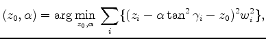
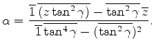
Now we define the best fitted intercept and curvature (
.
Now we define the best fitted intercept and curvature (
![]() and
and ![]() ) values as follows:
) values as follows:
| (16) |
 is the energy of the event at angle
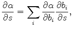
It is easy to find
 on
on 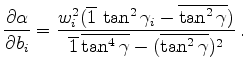 |
(18) |
 are defined respectively in equations (17) and (10).
|
|
|
|
Moveout-based wave-equation migration velocity analysis |