A new waveform inversion workflow: Application to near-surface velocity estimation in Saudi Arabia

Field data application

Our new workflow was applied to a 2D land dataset acquired in Saudi Arabia. The line geometry and the stacked section of the 2D data are shown in Figure 5. The section of the line used for waveform inversion is between the two vertical red lines. The acquisition geometry was not strictly 2D, that is it was not in a straight line. The waveform inversion algorithm that was used is a 2D implementation of the time-domain approach described in Shen (2010). The line geometry was hence converted to 2D by a simple projection of the line onto the x-axis. The starting model was obtained by ray-based method using picked first-break traveltimes. Starting source wavelets were obtained by stacking part of the moved-out refractions, and vary from shot to shot. The source wavelets were then updated at each iteration of the inversion. We used a total of 110 shots, with 180m shot spacing and 30 m receiver spacing. Offset used for inversion ranged from -4000 to -400 m for each shot. The lowest frequency in the data was 10 Hz, which makes direct application of waveform-based inversion for the low frequencies of velocity difficult. Two waveform inversion runs were performed. The first run started directly from the first arrival traveltimes tomography model and the second run included an intermediate step of wave-equation traveltime inversion applied to the full bandwidth data.

geostack
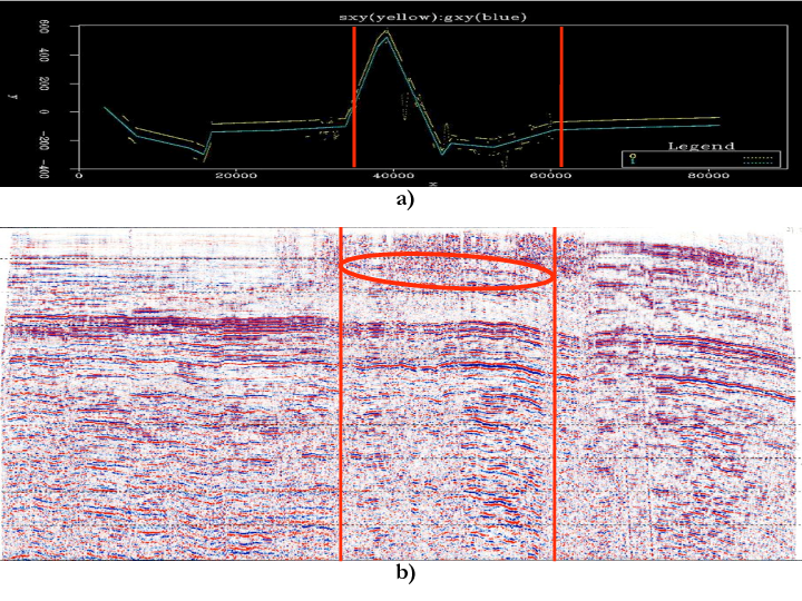
Figure 5. A land 2D data case showing a) the x,y source receiver geometry, and b) the stacked. The area for waveform inversion is between the vertical red lines. Blue indicates source, and yellow indicates receiver locations. [NR]

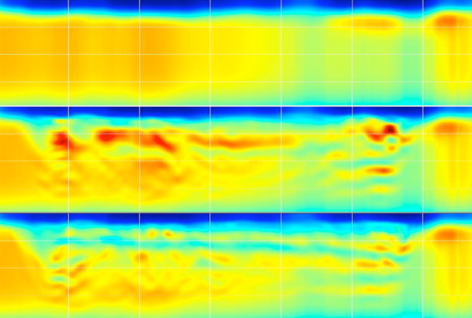
The starting model and final results are shown in Figure 6. The inversion result after the wave-equation traveltime inversion shows a continuous low velocity event in the upper middle portion of the section

threevel
Figure 6. Starting depth velocity model using ray-based tomography (top), and waveform inversion results without (middle) and with (bottom) wave-equation traveltime inversion. [NR]

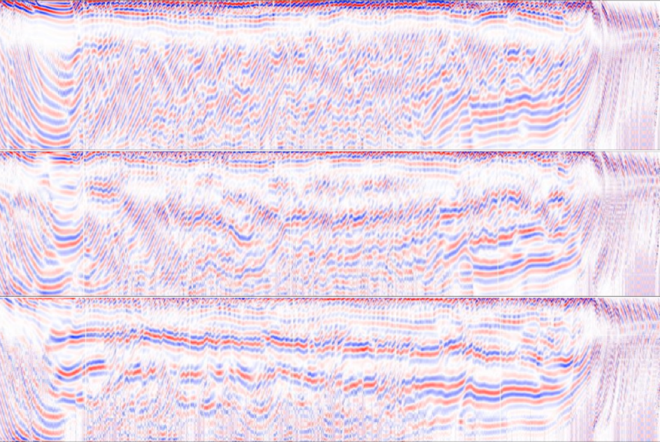
The reverse time migrated (RTM) images in Figure 7 clearly show that wave-equation traveltime inversion has improved the final image. Indeed, with better velocities, we get more spatial coherence, particularly in the neighborhood of the low velocity layer where reflections are seen both in the RTM result and on the stacked section in Figure 5 (indicated by the red ellipse).

threeimg
Figure 7. RTM images corresponding to the starting depth velocity model using ray-based tomography (top), and to the waveform inversion results without (middle) and with (bottom) wave-equation traveltime inversion. [NR]

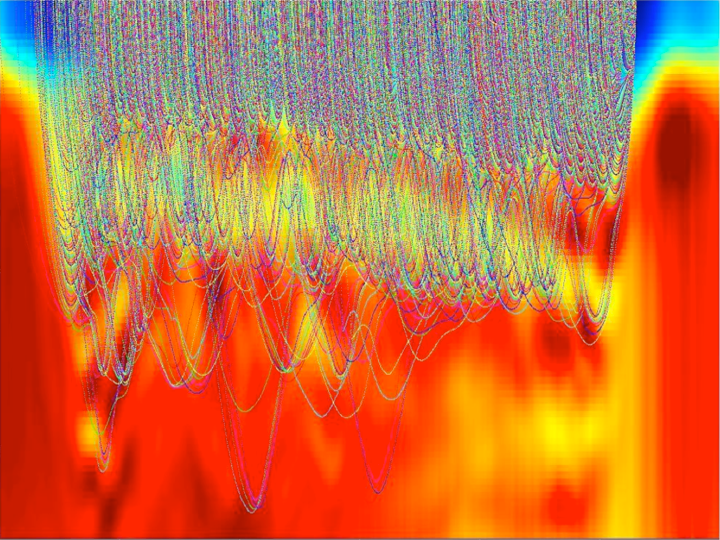
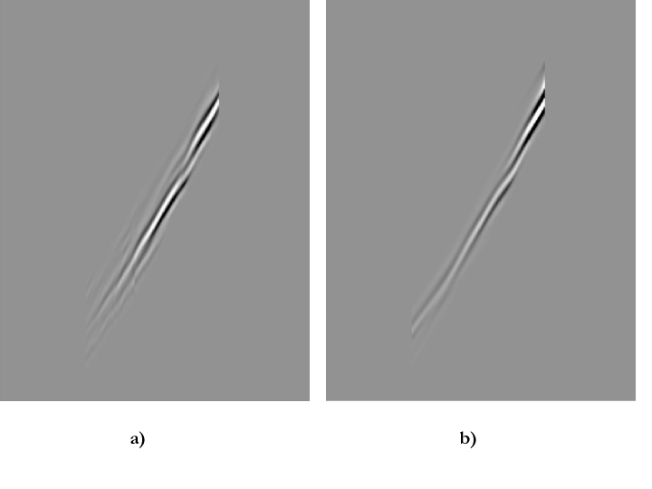
Figure 8 shows ray tracing through the final velocity model within the data offsets used for inversion. This display verifies the depth of the valid velocity model updates, which in this case confirmed that the low velocity layer is indeed the result of inversion rather than an artifact. Since we are matching waveforms, it is also important to compare the modeled data with the input refraction data (Figure 9). It can be seen that waveforms and traveltimes match quite well despite differences in absolute amplitude. However, these difference are not a problem for the waveform-based waveform inversion objective function proposed by Shen (2010). Based on these results, the wave-equation traveltime inversion step seems to considerably improve the final results. This improvement could also be explained by the fact that the ray-based model was not totally consistent with the waveform inversion algorithm used.

realray
Figure 8. Ray tracing through the final velocity model. This shows that low velocity layer is indeed from inversion instead of being an artifact. [NR]

realcomp
Figure 9. Comparison of a) input and b) modeled refractions. Note the similar kinematics despite minor differences in absolute amplitudes. [NR]

A new waveform inversion workflow: Application to near-surface velocity estimation in Saudi Arabia