An approximation of the inverse Ricker wavelet as an initial guess for bidirectional deconvolution

introduction

Zhang and Claerbout (2010) proposed a new method for blind deconvolution to overcome the minimum-phase assumption, called ``bidirectional deconvolution''. A seismic data trace can be represented by a convolution of a wavelet with a reflectivity series,

$$d = r * w,$$ (1)

where $d$ denotes the seismic data trace, $r$ denotes the reflectivity series, and $w$ denotes a wavelet.

In conventional blind deconvolution, we assume that $w$ is a minimum-phase wavelet. However this assumption is not applicable for field seismic data. If $w$ denotes a mixed-phase wavelet, it can be represented by a convolution of two parts: $w = w_a*w_b^r$ , where $w_a$ is a minimum-phase wavelet and $w_b$ is a reversed minimum-phase wavelet; hence $w_b^r$ itself is a maximum-phase wavelet. (The superscript r denotes reversed in time.) Thus equation 1 can be rewritten as

$$d = r*(w_a *w_b ^r ).$$ (2)

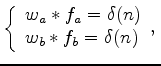
If we know the inverse filters $f_a$ and $f_b^r$ for $w_a$ and $w_b^r$ , respectively, to satisfy

$$\left\{ \begin{array}{l} w_a*f_a = \delta (n) \\ w_b*f_b = \delta (n) \end{array} , \right.$$ (3)

we can recover the reflectivity series:

$$r = d*f_a *f_b ^r,$$ (4)

where filter $f_a$ is the inverse signal of $w_a$ and filter $f_b$ is the inverse signal of $w_b$

Now we can use nonlinear inversion to solve this blind deconvolution problem for a mixed-phase wavelet by solving the two equations below alternately:

$$\left\{ \begin{array}{l} (d*f_b^r)*f_a = r_a \\ (d*f_a)^r*f_b=r_b^r \end{array} \right.$$ (5)

where both $f_a$ and $f_b$ are minimum-phase signals.

Shen et al. (2011) proposed another method to solve equation 4. Instead of solving for $f_a$ and $f_b$ alternately, they solve $f_a$ and $f_b$ simultaneously. Using this new approach allows us to estimate results with similar waveforms for $f_a$ and $f_b$ , which is a natural characteristic for data with a Ricker-like wavelet. In addition, this new method is faster than previous one. Hence we will use this to perform bidirectional deconvolution.

Since bidirectional deconvolution is a nonlinear problem, it requires that the starting model be close to the true one, and it is highly sensitive to the initial guess for both $f_a$ and $f_b$ . Shen et al. (2011) uses a simple one-spike impulse function for both filters. However, sometimes the true model does not resemble an impulse function. Therefore, we attempt to find a better initial guess.

An approximation of the inverse Ricker wavelet as an initial guess for bidirectional deconvolution