Elastic wavefield directionality vectors

P-wave and S-wave amplitude separation and displacement decomposition

The Helmholtz amplitude separation is based on the assumption that any vector field can be described as resulting from a combination of a scalar and vector potential fields:

$$\bold U = \nabla \Phi + \nabla \times \bold \Psi,$$ (4)

Where $\Phi$ is the scalar potential field and $\bold \Psi$ is the vector potential. $\bold U$ is the elastic displacement vector wavefield. The scalar potential generates pressure waves, and the vector potential generates shear waves. Therefore, the Helmholtz method of separating the P-wave amplitude from the S-wave amplitude is to apply a divergence operator and a curl operator to the displacement field:

$$P = \nabla \cdot \bold U = \nabla^2 \Phi;$$ (5)

$$\bold S = \nabla \times \bold U = -\nabla^2 \Psi.$$ (6)

The derivation of P-wave and S-wave displacement decomposition by Zhang and McMechan (2010) is done in the wavenumber domain. For an isotropic medium, the linear equation system they arrive at is:

$$\bold K \times \bold {\tilde U^P} = 0,$$ (7)

$$\bold K \times \bold {\tilde U} = \bold K \times \bold {\tilde U^S},$$ (8)

$$\bold K \cdot \bold {\tilde U^S} = 0,$$ (9)

and

$$\bold K \cdot \bold {\tilde U} = \bold K \cdot \bold {\tilde U^P},$$ (10)

where $\bold {\tilde U}$ is the 3D spatial fourier transform of the displacement field $\bold {\tilde U} = ( \tilde U_x, \tilde U_y, \tilde U_z )$ . $\bold {\tilde U^P}$ and $\bold {\tilde U^S}$ are the unknown P and S displacements. $\bold K = ( K_x, K_y, K_z )$ is the wavenumber vector that describes the particle displacement direction. $K_i = \frac {\omega}{V_i}$ , where $V_i$ is the phase velocity in the $i$ direction, and $\omega$ is angular frequency.

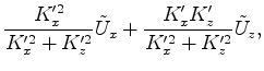
The solutions for P-wave displacements of these systems in 2D are:

$$\tilde U^P_x = K^2_x \tilde U_x + K_x K_z \tilde U_z,$$ (11)

$$\tilde U^P_z = K^2_z \tilde U_z + K_z K_x \tilde U_x.$$ (12)

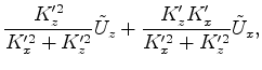
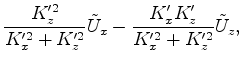
The solutions for S-wave displacements are:

$$\tilde U^S_x = K^2_z \tilde U_x - K_x K_z \tilde U_z,$$ (13)

$$\tilde U^S_z = K^2_x \tilde U_z - K_z K_x \tilde U_x.$$ (14)

It is important to note that the $K$ in these equations is normalized by the absolute value of the wavenumber $\left \vert \bold K \right \vert$ . Therefore, if we use $K'$ to designate the non-normalized wavenumbers, each wavenumber must be divided by $\frac{1}{\sqrt {K'^2_x + K'^2_z}}$ . Equations 12 - 14 then take the form:

$$\tilde U^P_x = \frac{K'^2_x}{K'^2_x + K'^2_z} \tilde U_x + \frac{K'_x K'_z}{K'^2_x + K'^2_z} \tilde U_z,$$ (15)

$$\tilde U^P_z = \frac{K'^2_z}{K'^2_x + K'^2_z} \tilde U_z + \frac{K'_z K'_x}{K'^2_x + K'^2_z} \tilde U_x,$$ (16)

$$\tilde U^S_x = \frac{K'^2_z}{K'^2_x + K'^2_z} \tilde U_x - \frac{K'_x K'_z}{K'^2_x + K'^2_z} \tilde U_z,$$ (17)

$$\tilde U^S_z = \frac{K'^2_x}{K'^2_x + K'^2_z} \tilde U_z - \frac{K'_z K'_x}{K'^2_x + K'^2_z} \tilde U_x.$$ (18)

As mentioned previously, these are decomposition operators for isotropic media only. I decided to use them initially, in order to evaluate the possibility of using elastic wavefield directionality for the purposes of angle gather creation. The main difference between displacement decomposition and the Helmholtz amplitude separation is that the decomposition is reversible. The sum of the decomposed P and S displacement vectors will result in the original pre-decomposed displacements. However, there is no theoretical way to go from the separated P and S amplitude fields back to the original displacement fields from which they were calculated.

Elastic wavefield directionality vectors