Reverse-time migration using wavefield decomposition

Examples with complex 2-D model

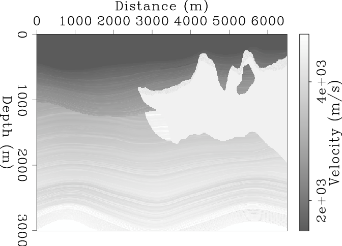
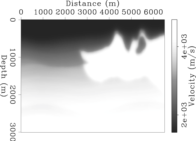
Figure 11(a) shows a complex 2-D velocity model windowed from the SEAM model. This model is used for modeling a 2-D synthetic data set, which contains 69 shot profiles. This data set involves the deployment of a 1-D array of regularly spaced geophones (every 20 meters) on the entire surface. For each shot record, a source is exploded on the surface with 80-meter shot spacing. In the pre-migration process, muting head waves and diving waves is appied to this data set. However, SRM elimination is not implemented. For RTM, the smoothed velocity in Figure 11(b) is used.

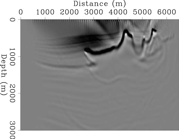
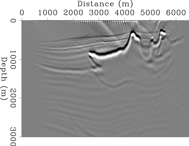
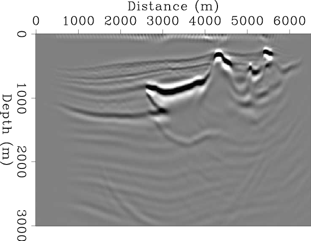
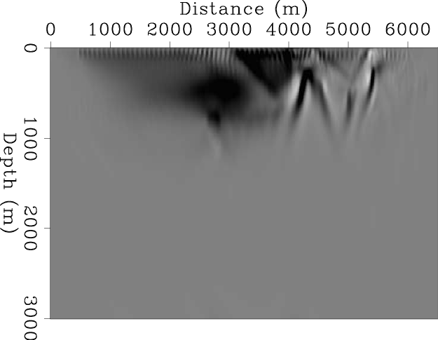
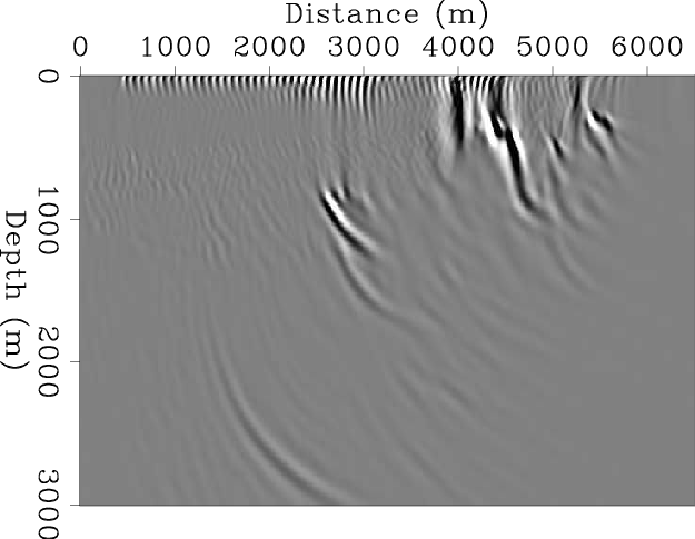
Figure 12(a) illustrates a conventional RTM image using the cross-correlation imaging condition in Equation 1, whereas Figure 12(b) shows the same image after applying a causal low-cut filter. We can see that RTM artifacts are partially attenuated using the low-cut filter.

vel1,vel1-mig
Figure 11. (a) A 2-D velocity model windowed from the SEAM model. (b) The smoothed velocity model used as the migration velocity.

crtm0-v1,crtm0-v1-lowcut
Figure 12. (a) A conventional RTM image of an entire 2-D synthetic data set using the cross-correlation imaging condition in Equation 1. (b) A causal low-cut filtered result of the image in (a).

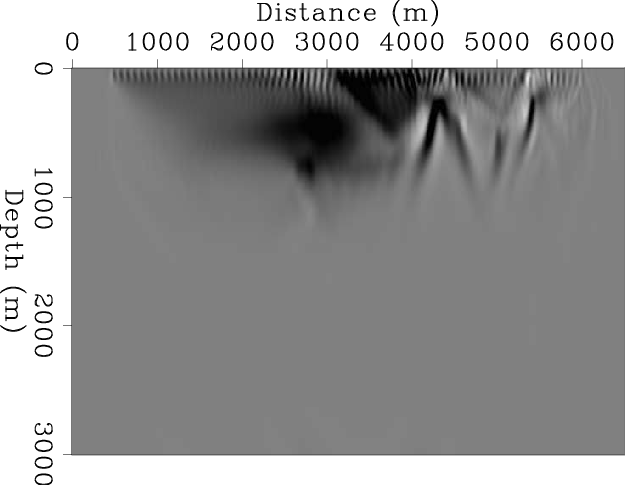
Figures 13(a) to 13(d) illustrate the vertically decomposed RTM images corresponding to the four decomposed images on the right-hand side of Equation 7. Figure 13(b) results from the upgoing source and downgoing receiver wavefields. This figure contains artifacts at shallow depths which have the same origin as those in Figure 8(b).

Figure 13(e) illustrates the RTM images the vertical backscatter-based imaging condition. As shown in the figure, the illumination of steeply dipping reflectors is poor. In contrast, Figure 13(f) represents the decomposed images from the decomposed source and receiver wavefields that have been propagated in vertically opposite directions.

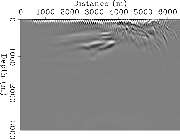
On the other hand, Figures 14(a) to 14(d) show the four different decomposed RTM images based on horizontal propagation directions of source and receiver wavefields. We can see that Figures 14(a) and 14(b) illustrate not only the images of steeply dipping reflectors but also artifacts in the shallow parts. These artifacts have the same origin as those in Figure 9(e).

Figure 14(e) is the result of using the imaging condition in Equation 9, i.e. the horizontal imaging condition. As shown in the figure, this imaging condition can image steeply dipping reflectors to an extent; however, most of low-angle reflectors cannot be imaged. In contrast, Figure 14(f), which involves the cross-correlation of the decomposed source and receiver wavefields caused by horizontally forward-scattered events, contains the major artifacts in the shallow parts of the model and the images of low-angle reflectors.

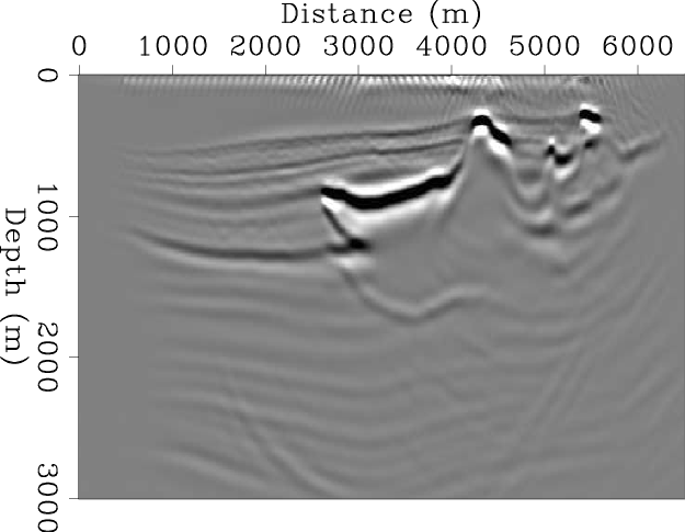
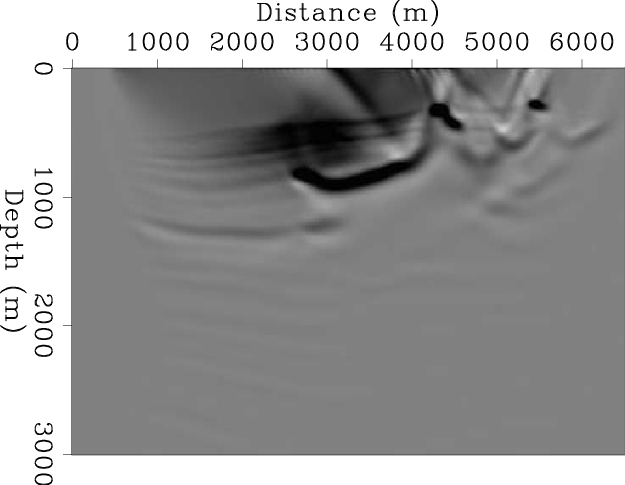
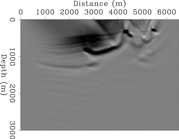
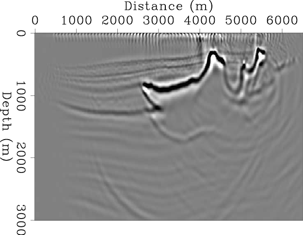
Figure 15 illustrates the result of using the Cartesian backscatter-based imaging condition, i.e. Equations 10. As shown in the figure, the result has the benefits of both vertical and horizontal imaging conditions. Both steeply dipping and low-angle reflectors are well imaged. In addition, Figure 15 contains artifacts in the shallow parts as a result of Figures 13(b), 14(a), and 14(b). However, strong RTM artifacts have significantly been attenuated.

It can be seen that the RTM image (Figure 15) using the Cartesian backscatter-based imaging condition, as in Equation 10, contains less strong artifacts compared to the conventional RTM image (Figure 12(a)) and the low-cut filtered RTM image (Figure 12(b)).

Thus, the combination of the vertical and horizontal imaging conditions is an effective technique for attenuating typical RTM artifacts, especially for complex velocity models. However, further investigation is necessary for removing the remaining artifacts in the shallow parts of the migrated images.

A possible solution is to modify the F-K filters in Equations 11 to 14, so there is no overlap between the decomposed wavefields with opposite propagation directions. In this study, I also tried using fan filters to decompose wavefields in the F-K domain. These filters aimed to limit the aperture of propagation directions of wavefields. However, as a result of the FFT of discontinuous functions, there still remained the overlap between the decomposed wavefields with opposite propagation directions.

v1-SdRu,v1-SuRd,v1-SdRd,v1-SuRu,v1-SdRuPSuRd,v1-SdRdPSuRu
Figure 13. Different vertically decomposed RTM images from 2-D synthetic data along with the smoothed migration velocity in Figure 11(b): (a) using the downgoing source and upgoing receiver wavefields, (b) using the upgoing source and downgoing receiver wavefields, (c) using the downgoing source and downgoing receiver wavefields, and (d) using the upgoing source and upgoing receiver wavefields. (e) The sum of the images (a) and (b) equivalent to Equation 8. (f) The sum of the images (c) and (d).

v1-SrRl,v1-SlRr,v1-SrRr,v1-SlRl,v1-SrRlPSlRr,v1-SrRrPSlRl
Figure 14. Different horizontally decomposed RTM images from 2-D synthetic data along with the smoothed migration velocity in Figure 11(b): (a) using the rightgoing source and leftgoing receiver wavefields, (b) using the leftgoing source and rightgoing receiver wavefields, (c) using the rightgoing source and rightgoing receiver wavefields, and (d) using the leftgoing source and leftgoing receiver wavefields. (e) The sum of the images (a) and (b) equivalent to Equation 9. (f) The sum of the images (c) and (d).

v1-vertPhoriz Figure 15. The RTM image from the Cartesian backscatter-based imaging condition as in Equation 10, i.e. the sum of Figure 13(e) and Figure 14(e).

Reverse-time migration using wavefield decomposition