|
|
|
|
A log spectral approach to bidirectional deconvolution |
A minimum phase wavelet can be made from any causal wavelet by
taking it to Fourier space, and exponentiating.
The proof is straightforward:
Let
![]() be the
be the ![]() transform
(
transform
(
![]() )
of any causal function.
Then
)
of any causal function.
Then ![]() will be minimum phase.
Although we would always do this calculation in the Fourier domain, the easy proof is in the
time domain. The power series for an exponential
will be minimum phase.
Although we would always do this calculation in the Fourier domain, the easy proof is in the
time domain. The power series for an exponential
![]() has no powers of
has no powers of ![]() ,
and it always converges because of the powerful influence of the denominator factorials.
Likewise
,
and it always converges because of the powerful influence of the denominator factorials.
Likewise ![]() , the inverse of
, the inverse of ![]() , always converges and is causal.
Thus both the filter and its inverse are causal. Q.E.D.
, always converges and is causal.
Thus both the filter and its inverse are causal. Q.E.D.
We seek to find two functions, one strictly causal the other strictly anticausal
(nothing at ![]() ).
).
| (1) | |||
| (2) |
| (3) | |||
| (4) |
| (5) |
| (6) |
 , and
, and
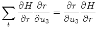
Take the gradient of the penalty function
assuming there is only one variable, ![]() giving a single regression equation:
giving a single regression equation:
 multiplies
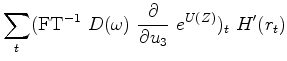
Equation (9) requires us to do an inverse Fourier transform
to find the gradient for only ![]() .
For
.
For ![]() there is an analogous expression,
but it is time shifted by
there is an analogous expression,
but it is time shifted by ![]() instead of
instead of ![]() .
Clearly we need only do one Fourier transform
and then shift it to get the time function required for other filter lags.
Thus the gradient for all nonzero lags is:
.
Clearly we need only do one Fourier transform
and then shift it to get the time function required for other filter lags.
Thus the gradient for all nonzero lags is:
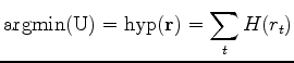
Equation (10) says if we were doing least squares,
the gradient would be simply the autocorrelation of the residual.
When the gradient at nonzero lags drops to zero, the residual is white.
Hooray! We long understood that limit.
What is currently new is that we now have a two-sided filter.
Likewise the ![]() limit must be where the output
is uncorrelated with the clipped output
at all lags but zero lag.
limit must be where the output
is uncorrelated with the clipped output
at all lags but zero lag.
(I'm finding it fascinating to look back on what we did all these years with the causal filter
![]() and comparing it to the non-causal exponential filter
and comparing it to the non-causal exponential filter ![]() .
In an
.
In an ![]() norm world for filter
norm world for filter ![]() we easily saw
the shifted output was orthogonal to the fitting function input.
For filter
we easily saw
the shifted output was orthogonal to the fitting function input.
For filter ![]() we easily see now the shifted output is orthogonal to the output.
The whiteness of the output comes easily with
we easily see now the shifted output is orthogonal to the output.
The whiteness of the output comes easily with ![]() but with
but with ![]() the Claerbout (2011) contains a lengthy and tricky proof of whiteness.)
the Claerbout (2011) contains a lengthy and tricky proof of whiteness.)
Let us figure out how a scaled gradient
![]() leads to a residual modification
leads to a residual modification
![]() .
The expression
.
The expression ![]() is in the Fourier domain.
We first view a simple two term example.
is in the Fourier domain.
We first view a simple two term example.
| (12) | |||
| (13) | |||
| (14) |
With that background, ignoring ![]() , and knowing the gradient
, and knowing the gradient
![]() ,
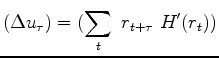
let us work out the forward operator to find
,
let us work out the forward operator to find
![]() .
Let ``
.
Let ``![]() '' denote convolution.
'' denote convolution.
iterate {
  alpha = - (Sum_i H'(r_i) dr_i ) / ( Sum H''(r_i) dr_i^2 )
  r = r + alpha dr
  }
In the pseudocode above, in the ![]() limit
limit ![]() and
and ![]() , so
so the first iteration gets the correct
, so
so the first iteration gets the correct ![]() , and
changes the residual accordingly so all subsequent
, and
changes the residual accordingly so all subsequent ![]() values are zero.
values are zero.
We are not finished
because we need to assure the constraint ![]() .
In a linear problem it would be sufficient to set
.
In a linear problem it would be sufficient to set
![]() ,
but here we soon do a linearization which breaks the constraint.
In the frequency domain the constraint is
,
but here we soon do a linearization which breaks the constraint.
In the frequency domain the constraint is
![]() .
We meet this constraint by inserting a constant
.
We meet this constraint by inserting a constant ![]() in equation (15)
and chosing
in equation (15)
and chosing ![]() to get
a zero sum over frequency of
to get
a zero sum over frequency of
![]() .
Let
.
Let ![]() denote a normalized summation over frequency.
By normalized, I mean
denote a normalized summation over frequency.
By normalized, I mean
![]() .
We must choose
.
We must choose ![]() so that
so that
![]() .
Clearly,
.
Clearly,
![]() .
Pick up again from equation
(15) including
.
Pick up again from equation
(15) including ![]() .
.
| (21) | |||
| (22) | |||
| (23) | |||
| (24) |
| (25) |
|
|
|
|
A log spectral approach to bidirectional deconvolution |