|
|
|
|
Migration velocity analysis for anisotropic models |
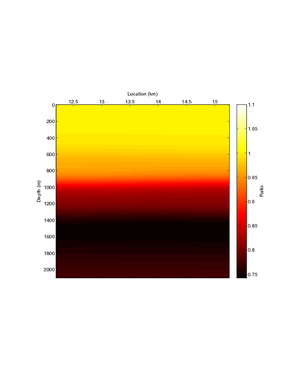
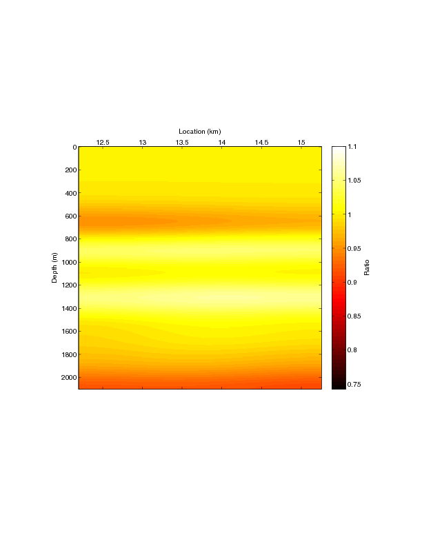
On the other hand, the ![]() update [Figure 2(d)] is in
general larger than the true
update [Figure 2(d)] is in
general larger than the true ![]() model [Figure
2(c)]. A trade-off is observed
below 1,600 m, where the inverted velocity is smaller but
model [Figure
2(c)]. A trade-off is observed
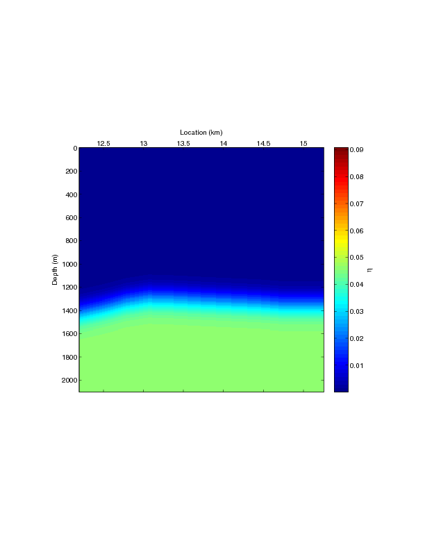
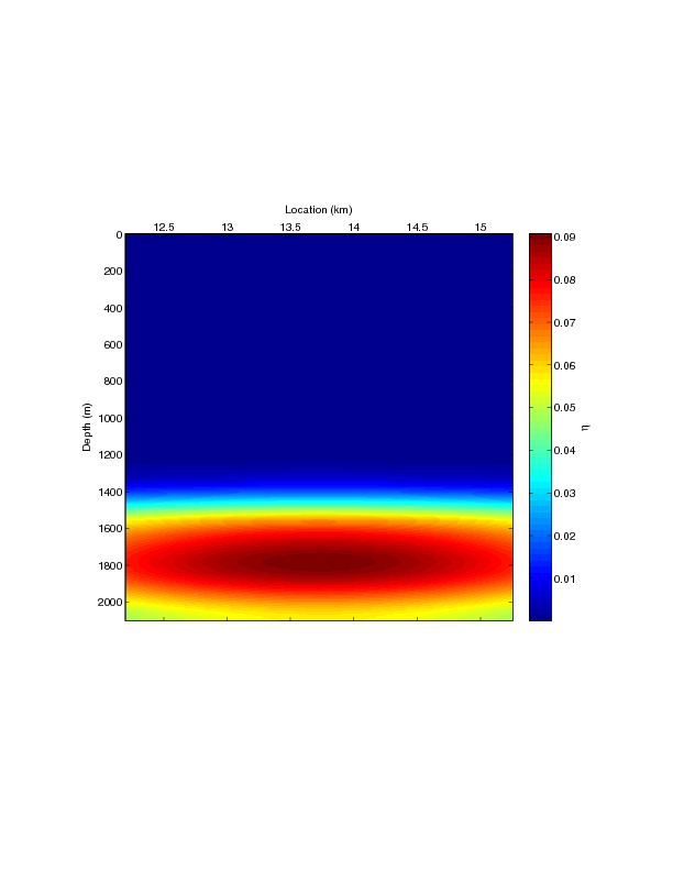
below 1,600 m, where the inverted velocity is smaller but ![]() is
much larger than the true values. This result illustrates the null space of
our inversion problem, since the reflector around 2,200 m is well-focused (although not perfectly focused) in the
final image obtained with the inverted model [Figure 3(b)]. This problem can presumably be
resolved by increasing the angle coverage at depth and allowing more
iterations in the inversion.
is
much larger than the true values. This result illustrates the null space of
our inversion problem, since the reflector around 2,200 m is well-focused (although not perfectly focused) in the
final image obtained with the inverted model [Figure 3(b)]. This problem can presumably be
resolved by increasing the angle coverage at depth and allowing more
iterations in the inversion.
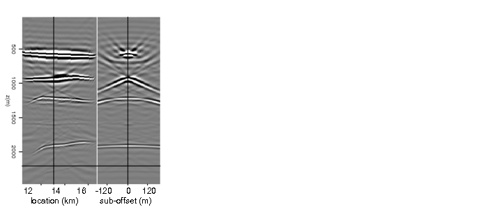
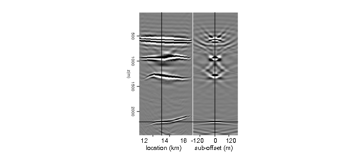
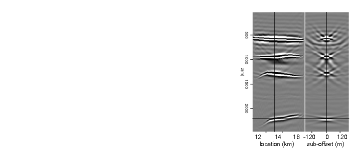
Figure 3 compares the subsurface-offset images using the initial model (a), the updated model (b), and the true model (c). After the inversion, the reflectors are focused at zero subsurface-offset, and the depths of the reflectors are closer to the true depths. The focused image shows that we are dealing with a non-linear problem with a large null space. To reduce the size of the null space, and hence the uncertainty in the inverted model, other information such as checkshots or rock-physics prior knowledge is needed (Li et al., 2011b,a).
|
|---|
|
init-over-true,inv-over-true,true-eta,inv-eta
Figure 2. (a) Ratio of initial velocity over true velocity; (b) ratio of inverted velocity over true velocity; (c) true |
|
|
|
|---|
|
init-image,final-image,true-image
Figure 3. Subsurface offset images using the initial model (a), the updated model (b), and the true model (c). |
|
|
|
|
|
|
Migration velocity analysis for anisotropic models |