Memory efficient 3D reverse time migration

GPU Implementation

Using the identical serial kernel in CUDA this propagation takes 18 minutes. This is slower than the fastest CPU technique because GPU global memory latency is higher than on the CPU, to harness the power of the GPU shared memory and registers must be used.

Micikevicius (2009) describes an efficient way of setting up the base wave propagation kernel that utilises latency hiding by copying stencil location values into shared memory, dependent on thread location. Performing this propagation in 3D is about 27 times faster than the naive GPU approach, with speeds of over 3 Gpts/s achievable for typical model dimensions, and a run time of 41s (for the previously used model).

Operations purely on GPU global memory are slower than on a CPU, with latencies of 400-600 cycles, rather than 100-200 on a CPU. Due to this, a typical school of thought minimises data manipulation on the GPU. This approach constitutes sending to host (CPU) the full 3D wavefield at each desired modeling time step, causing the CPU wavefield object to be 4D. This can then be transposed and windowed accordingly. This method gives a speed of 24x over the best, blocked and parallelised CPU equivalent. Having to copy data this way is a shortcoming of interacting Fortran90, C and CUDA.

Storing the entire 4D wavefield as an allocated object on the CPU is unwise - memory is quickly saturated. For example, a model size of 500x500x500 dictates that only 64 time steps could be performed (on a 4 Gb card).

Several improvements can be made to make the GPU propagation as fast as possible. A new windowing kernel can be used to only send 2D wavefield slices back to the host (corresponding to desired acquisition geometries), this only marginally slows down the modeling and makes the full implementation vastly more flexible. In fact since now less data has to copied back to the CPU a speed up of about 1.3x is seen.

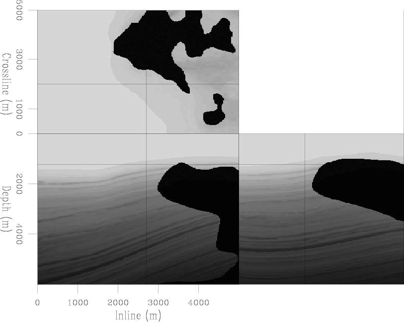
velslice3d
Figure 3. A 3D cubeplot of the velocity model used for 3D imaging

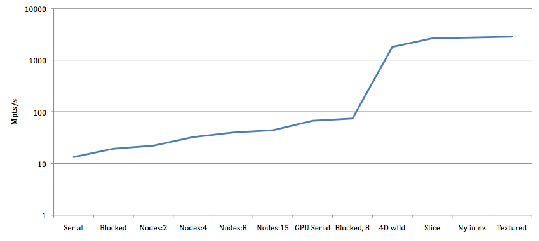
The final speed up thus far when compared to most efficient, blocked and parallelised CPU routine is about 35x, and the current throughput is about 2.2 Gpoints/s. If the CPU modeling was fully optimised the observed speed up would be 15-20x. The evolution of computation speed (measured in million computed points per second) against propagation scheme can be observed in Figure 4.

speed
Figure 4. Graphing the speed up between various CPU and GPU propagation schemes

The finite computational domain used when simulating wavefield propagation provides additional challenges. To accurately simulate real world physics, an infinite domain must be used, but of course this is not possible. If no boundary conditions are used then reflections from the computational domain are prevalent in the modeled data. There are many ways of reducing or hiding these domain reflections, such as zero value, zero order, absorbing, damping and Perfectly Matched Layer (PML) (Turkel and Yefet, 1998). For modeling an absorbtion scheme was used, which reduced throughput by about 10%.

This accelerated 3D wave propagation method will provide the engine for 3D RTM.

Memory efficient 3D reverse time migration