Combining forward-scattered and back-scattered wavefields in velocity analysis

Method

When linearized over slowness, the FWI gradient can be written as follows (Tarantola, 1984):

$$g(\mathbf x) = \sum_{\omega,\mathbf x_s,\mathbf x_r} -2 \omega^2 ... ...ega)G^*(\mathbf x,\mathbf x_r,\omega) \Delta d(\mathbf x_r,\mathbf x_s,\omega),$$ (1)

where $G$ is the Green's function, $\mathbf s_0$ is the background slowness, $\Delta d$ is the data residual, $\mathbf x_s$ and $\mathbf x_r$ are the source and receiver coordinates, $\mathbf x$ is the Green's functions' coordinate, and $\omega$ is frequency. FWI updates contain two components: a tomographic component and a migration component. To better understand these components, we will look at the migration and tomographic operators.

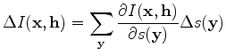
The operator relating the slowness model and the image is nonlinear. Therefore, the first step in evaluating a tomographic operator is to linearize the image $\mathbf I$ around the background slowness $\mathbf s_0$ , as follows:

$$\mathbf I = \mathbf I_0 + \frac{\partial \mathbf I}{\partial \mathbf s}\vert_{s_0}(\mathbf s - \mathbf s_0) + ...,$$ (2)

where $\mathbf I_0$ is the background image. Under the Born approximation, the background image can be obtained as follows:

$$\mathbf I_0 = \mathbf L^* \mathbf d ,$$ (3)

where $\mathbf L$ is the Born modeling operator, and its adjoint $\mathbf L^*$ is the migration operator. By neglecting the higher-order terms in the image series, we can define the tomographic operator as follows:

$$\Delta \mathbf I = \frac{\partial \mathbf I}{\partial \mathbf s}\vert_{s_0} \Delta \mathbf s = \mathbf T \Delta \mathbf s ,$$ (4)

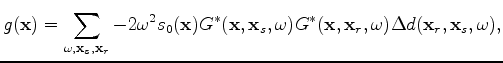
where $\mathbf T$ is the tomographic operator. Now, we use the conventional imaging condition as follows:

$$I(\mathbf x, \mathbf h) = \sum_{\omega,\mathbf x_s,\mathbf x_r} G... ...^*(\mathbf x + \mathbf h,\mathbf x_r,\omega) d(\mathbf x_r,\mathbf x_s,\omega),$$ (5)

where $I$ is the image, $d$ is the surface data, and $\mathbf h$ is the subsurface offset. The background image $I_0$ can be written as follows:

$$I_0(\mathbf x, \mathbf h) = \sum_{\omega,\mathbf x_s,\mathbf x_r}... ...^*(\mathbf x + \mathbf h,\mathbf x_r,\omega) d(\mathbf x_r,\mathbf x_s,\omega),$$ (6)

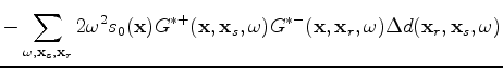
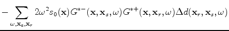
where $G_0$ is the background Green's function. After derivation, as shown in Almomin and Tang (2010), we obtain the forward tomographic operator as follows:

$$\Delta I(\mathbf x, \mathbf h) = \sum_{\mathbf y} \frac{\partial I(\mathbf x, \mathbf h)}{\partial s(\mathbf y)} \Delta s(\mathbf y)$$

$$= \sum_{\omega,\mathbf x_s,\mathbf x_r,\mathbf y} \left\lbrace-2 ... ...hbf h,\mathbf x_r,\omega) d(\mathbf x_r,\mathbf x_s,\omega) \Delta s(\mathbf y)$$

$$+ \sum_{\omega,\mathbf x_s,\mathbf x_r,\mathbf y} \left\lbrace-2 ... ...bf y,\mathbf x_r,\omega) d(\mathbf x_r,\mathbf x_s,\omega) \Delta s(\mathbf y),$$ (7)

where $\mathbf y$ is the slowness coordinate. Notice that all the Green's functions in the migration and tomographic operators are background Green's functions, which means that they do not contain any perturbations. Thus, the migration operator correlates two background wavefields, whereas the tomographic operator correlates a background and a perturbed wavefield. Therefore, a migration component can be generalized as the result of correlating wavefields moving in the opposite direction, whereas a tomographic component is the result of correlating wavefields moving in the same direction. In FWI, the background and perturbed wavefields are summed together in one wavefield. Nonetheless, these components are correlated together to compute the gradient.

wemva26deltaS,wemva26deltaSfk
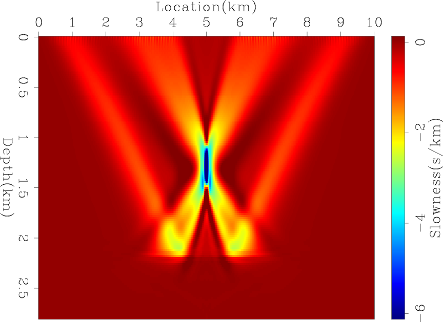
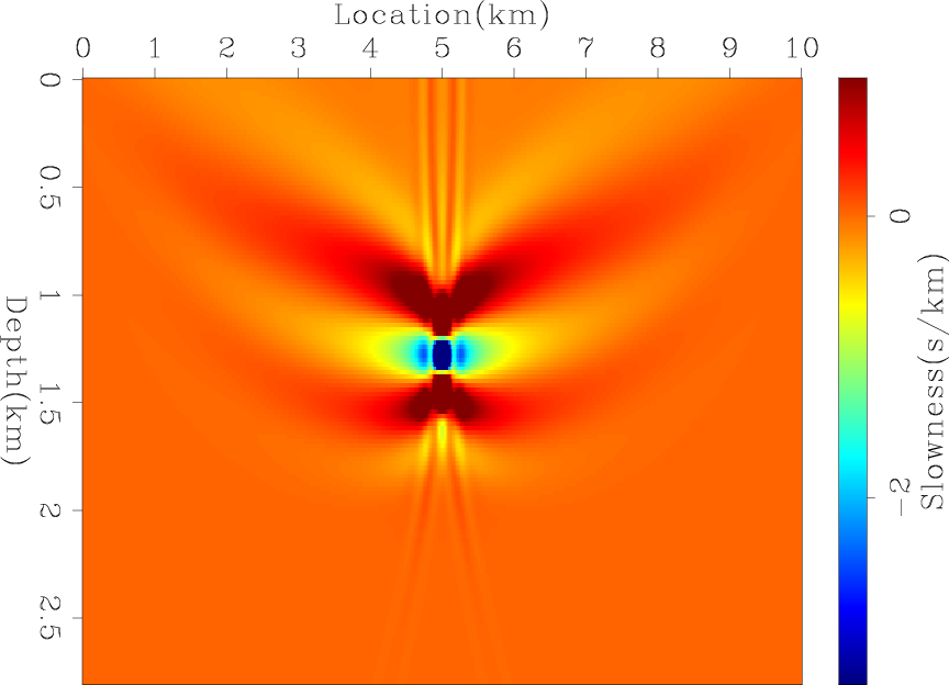
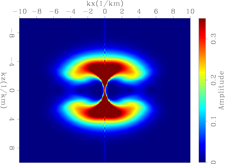
Figure 1. The tomographic operator response (a) and its amplitude spectrum (b).

wemva27imaged,wemva27imagedfk
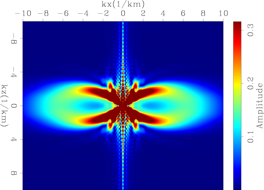
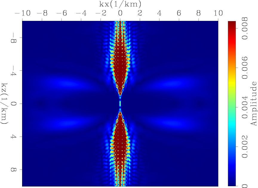
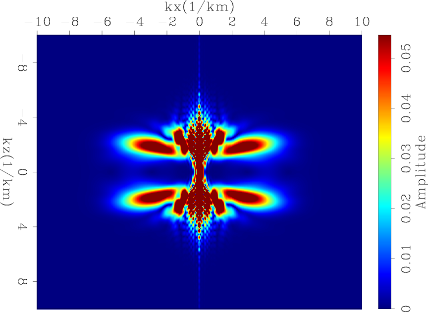
Figure 2. The migration operator response (a) and its amplitude spectrum (b).

I now compute the operators' responses in a surface acquisition. The receiver spacing is 20 m, the source spacing is 80 m, and the temporal sampling is 2 ms. Figure 1(a) shows the tomographic operator response by applying its forward and adjoint on a spike. This operator response represents one column of the Hessian matrix of the tomographic operator. Figure 1(b) shows the amplitude spectrum of the tomographic operator response, which shows that the tomographic updates illuminate only the very small vertical wavenumbers. Similarly, figure 2(a) shows the migration operator response of a spike, and figure 2(b) shows its amplitude spectrum. Unlike the tomographic component, the migration component illuminates larger vertical wavenumbers. The illuminated wavenumbers in both operators depend on the reflection angles as well as the frequency content of the data. In this case, the data was created with a Ricker wavelet that has a dominant frequency of 15 Hz.

Now that I have defined the components in FWI, we can take a closer look at their error sensitivity. The migration operator is linear with respect to model updates. Hence, the migration component in FWI also behaves in a linear sense. This can be better explained by observing that wavefields moving in opposite directions are always going to result in the correct sign of update, as long as the source wavelet is correct. Background velocity changes, or errors, will mostly affect the position at which the wavefields correlate. On the other hand, tomographic components correlate wavefields that are moving in the same direction. For the correlation to have the correct direction, the two wavefields should be within the wavelength of one another. This strict requirement causes the nonlinear behavior of FWI. Since WEMVA techniques do not have such a requirement, they tend to have more stable behavior when the velocity error is large. Our goal is to combine the robust components of FWI and WEMVA.

One way to decompose the FWI gradient into its tomographic and migration components is to separate the wavefields based on their direction of propagation, e.g. up or down, which can be done in Fourier domain (Hu and McMechan, 1987; Liu et al., 2007; Taweesintananon, 2011). The decomposed FWI gradient can be written as follows:

$$g(\mathbf x) = - \sum_{\omega,\mathbf x_s,\mathbf x_r} 2 \omega^2 s_0(\mathbf x)... ...a)G^{*-}(\mathbf x,\mathbf x_r,\omega) \Delta d(\mathbf x_r,\mathbf x_s,\omega)$$

$$- \sum_{\omega,\mathbf x_s,\mathbf x_r} 2 \omega^2 s_0(\mathbf x)... ...a)G^{*+}(\mathbf x,\mathbf x_r,\omega) \Delta d(\mathbf x_r,\mathbf x_s,\omega)$$

$$- \sum_{\omega,\mathbf x_s,\mathbf x_r} 2 \omega^2 s_0(\mathbf x)... ...a)G^{*-}(\mathbf x,\mathbf x_r,\omega) \Delta d(\mathbf x_r,\mathbf x_s,\omega)$$

$$- \sum_{\omega,\mathbf x_s,\mathbf x_r} 2 \omega^2 s_0(\mathbf x)... ...)G^{*-}(\mathbf x,\mathbf x_r,\omega) \Delta d(\mathbf x_r,\mathbf x_s,\omega),$$ (8)

where the positive and negative superscript signs of $G$ indicate the direction of propagation of the wavefield.

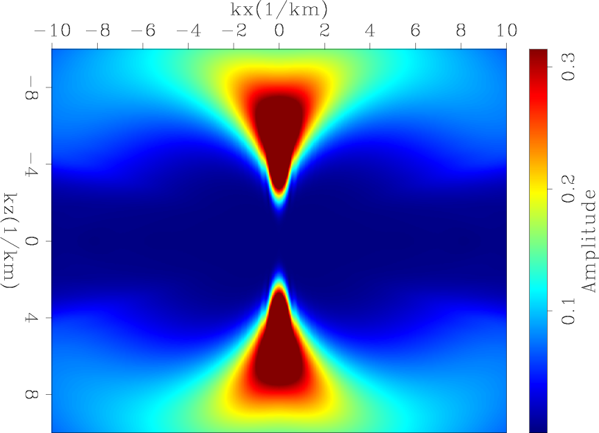
In order for the migration component of FWI gradient to improve the convergence and results of WEMVA gradient, the two need to have some overlap of their illuminated wavenumbers. Figure 4(a) shows the multiplication of the amplitude spectra in 1(b) and 2(b). The overlap seems to be only at very low horizontal wavenumbers, which have some truncation artifacts. However, the operator's response is a function of frequency. Therefore, by taking lower frequencies when computing the migration component, we may increase the overlap region of the two gradients.

wemva27imagedlf,wemva27imagedlffk
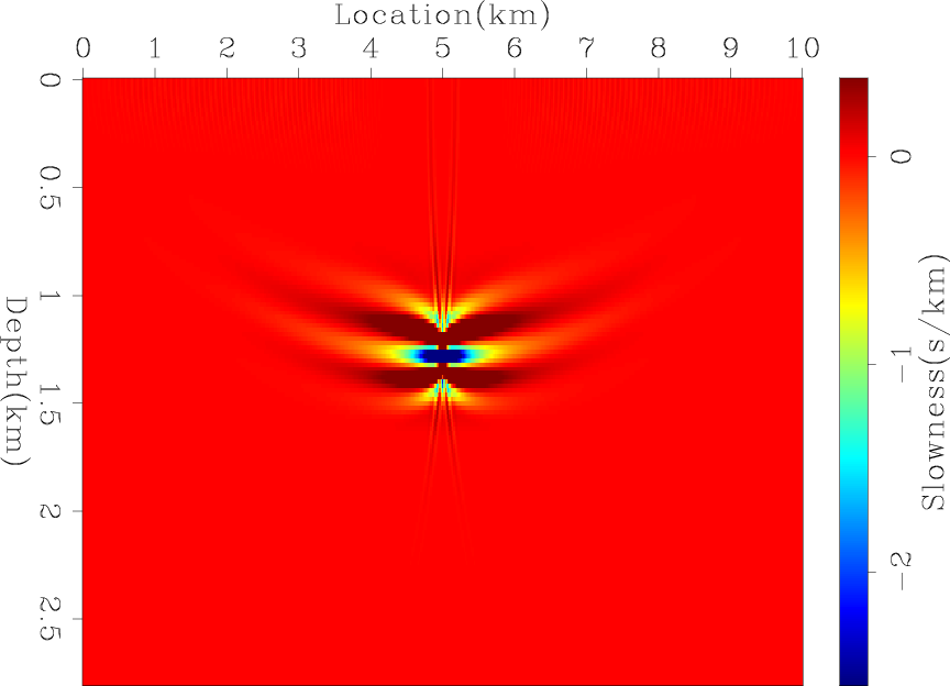
Figure 3. The low-frequency migration operator response (a) and its amplitude spectrum (b).

wemva27deltaSmfk0,wemva27deltaSmfk
Figure 4. The spectra product of the tomographic operator with (a) the migration operator and (b) the low-frequency migration operator.

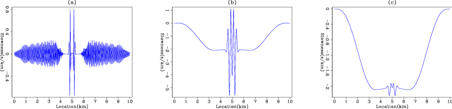
wemva27stacks
Figure 5. The vertical stack of (a) migration operator response, (b) low-frequency migration operator response and (c) laterally smooth low-frequency migration operator response.

Figure 3(a) shows the migration operator response of a spike with a 5 Hz Ricker wavelet, and figure 3(b) shows its amplitude spectrum. With lower frequencies, the migration operator response shifts toward smaller vertical wavenumbers. Figure 4(b) shows the multiplication of the amplitude spectra in 1(b) and 3(b), which shows a much larger and stronger overlap compared to figure 4(a). Figure 5 shows the vertical average migration response at 15 Hz and 5 Hz. It is clear that at low frequencies, the migration update starts to have small vertical-wavenumber contribution.

Combining forward-scattered and back-scattered wavefields in velocity analysis