Correlation-based wave-equation migration velocity analysis

Modified correlation-based WEMVA

There were two disadvantages to the original correlation-based WEMVA gradient. First, it assumes a single correlation lag per trace. Second, it is sensitive to the actual values of the picked correlation lags. If these lags are not correct, the gradient might have a cycle-skipping problem. In order to overcome these disadvantages, I approximate the shifted flat image by the observed image to get the following modified gradient:

$$\nabla J = \sum_{z} \left( \frac{\partial I_{\text {obs}}(z, \gam... ...\frac{\partial}{\partial z} I_{\text {obs}}(z, \gamma; \mathbf x) \frac{\xi}{E}$$ (11)

This modified gradient is immune to cycle-skipping since the residual and operator match by design. In addition, it is not as sensitive to the values of the picked lags. Finally, multiple picked lags could be used in this formulation.

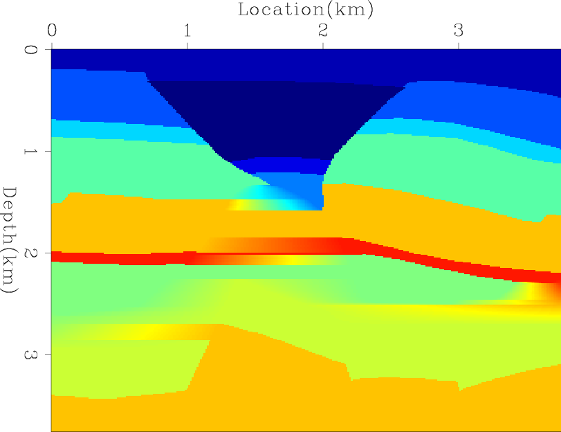
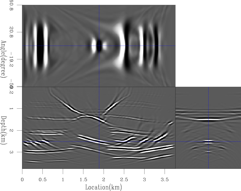
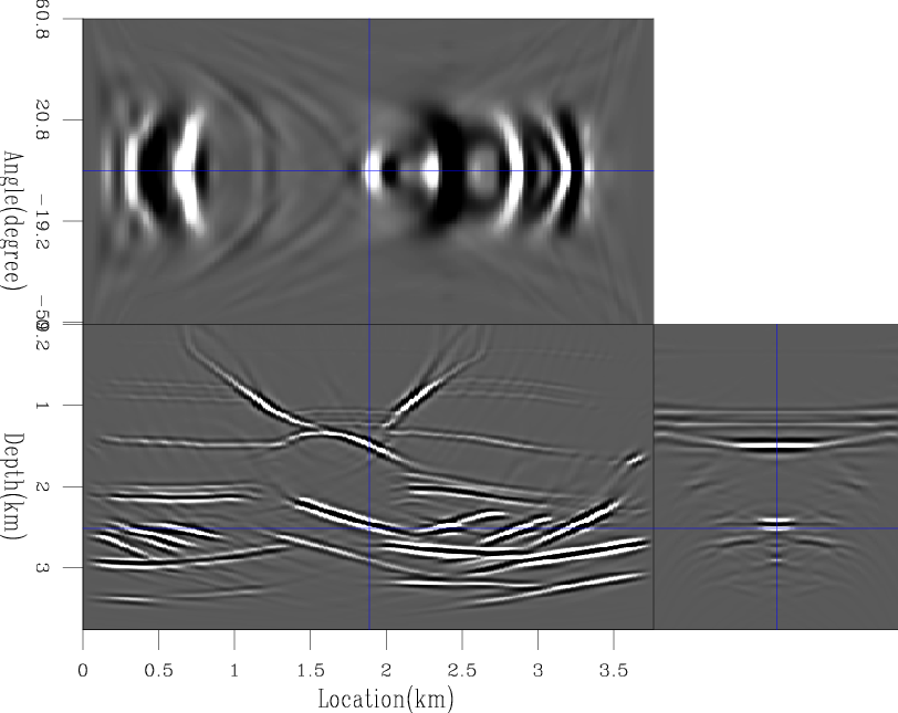
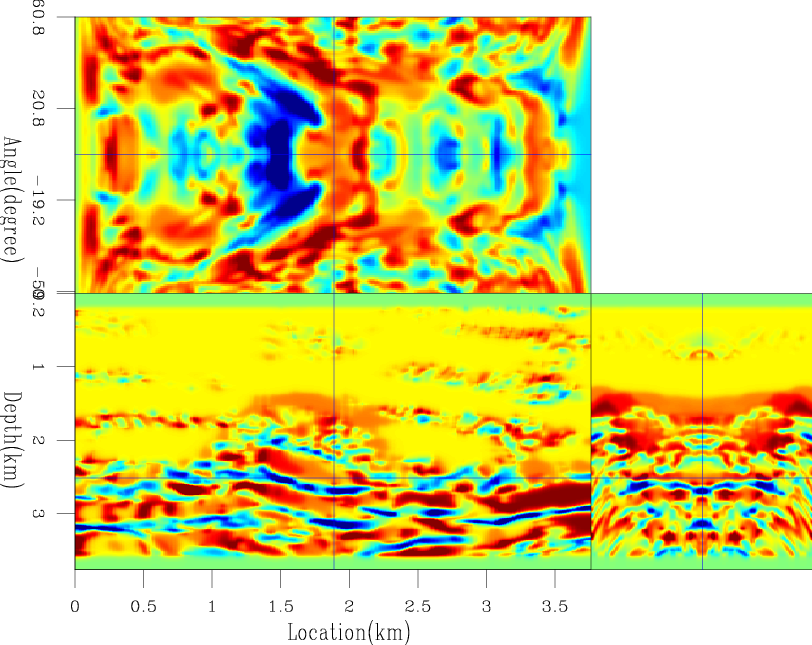
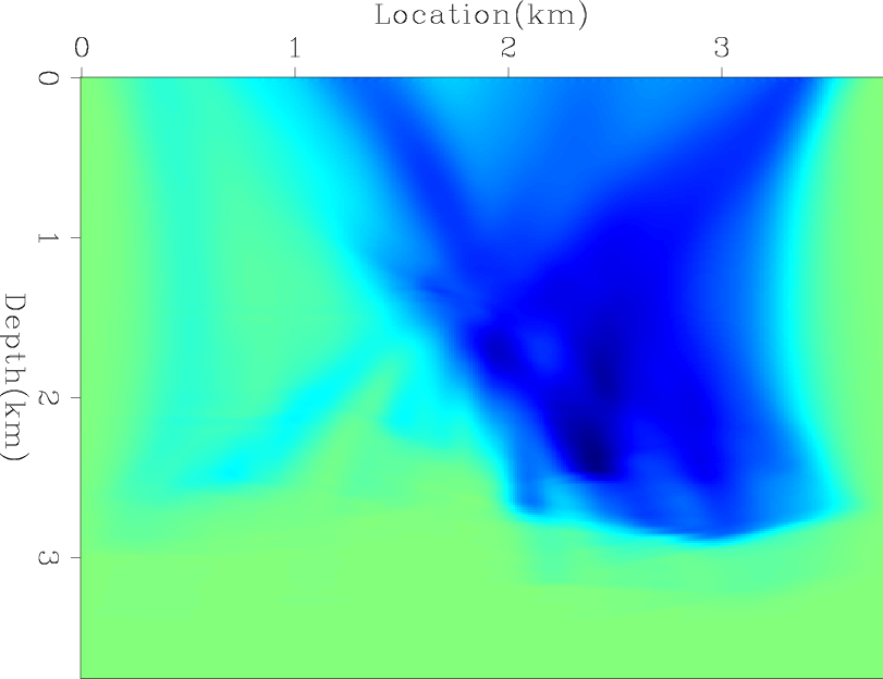
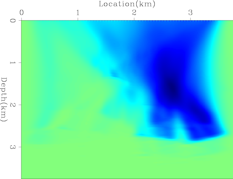
Figures 3(a) and 3(b) show the true and background velocities of a salt model. ADCIGs using these two velocities on the observed data are shown in figures 4(a) and 4(b). Next, I used a sliding Gaussian window to compute and pick local cross-correlation panels between the observed image and the stacked image. Then, I picked the maximum correlation lag at each depth level. The picked lags are shown in figure 5.

wemva22truev,wemva22bgv
Figure 3. The true velocity salt model (a) and the background velocity model (b).

wemva22adcigtv,wemva22adcigbgv
Figure 4. ADCIGs using the true velocity salt model (a) and using the background salt model (b).

wemva22lags3dc
Figure 5. Lag estimation of the maximum local correlation.

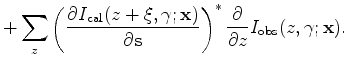
As in the previous example, I computed the optimum gradient using the true velocity anomaly and the modified correlation-based WEMVA gradient using the picked correlation lags. These two gradients are shown in figure 6(a) and 6(b). Although we used the apparent depth of the stacked image, the modified gradient shows very good results that are very similar to the optimum gradient. In this case, the velocity information in large reflection angles was more dominant than those in zero reflection angle.

wemva22amacoopt,wemva22amacoz
Figure 6. The optimum WEMVA gradient of the salt model (a) and the modified correlation-based WEMVA gradient of the salt model (b).

Correlation-based wave-equation migration velocity analysis