|
 |
 |
 | Correlation-based wave-equation migration velocity analysis |  |
![[pdf]](icons/pdf.png) |
Next: Synthetic Examples
Up: Almomin: WEMVA
Previous: Introduction
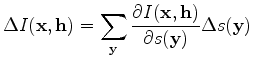
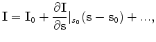
The first step in evaluating a tomographic operator is to linearize the image  around the background slowness
 , as follows:
 |
(1) |
where
 is the background image and
  is the slowness model. By neglecting the higher order terms in the image series, we can define the tomographic operator as follows:
 |
(2) |
where 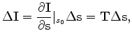 is the tomographic operator. Now, we use the conventional imaging condition as follows:
 |
(3) |
where 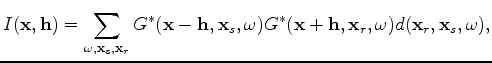 is the image,
  is the Green's function,
  is the surface data,
  is frequency,
 and
are the source and receiver coordinates, and
and
are the source and receiver coordinates, and  is the subsurface offset. To evaluate the tomographic operator
, I take the derivative of the imaging condition as follows:
is the subsurface offset. To evaluate the tomographic operator
, I take the derivative of the imaging condition as follows:
where  is the slowness coordinate. The full derivation of the tomographic operator is presented in Almomin and Tang (2010).
After defining the tomographic operator, I use a cross-correlation function to estimate image perturbations:
 |
(5) |
where 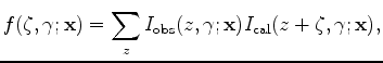 is the lag,
  is the reflection angle,
  is the surface coordinates,
  is depth,
 is the angle-domain image using the observed data, and
 is the angle-domain image using the calculated data, which is modeled with the background slowness.
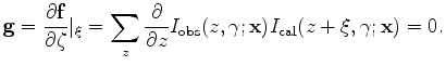
is always going to be flat, since I create Born-modeled data using a reference model as the reflectivity and the background slowness and then migrate that data using the same background slowness. Next, I define
is the angle-domain image using the calculated data, which is modeled with the background slowness.
is always going to be flat, since I create Born-modeled data using a reference model as the reflectivity and the background slowness and then migrate that data using the same background slowness. Next, I define  to be the lag that maximizes the correlation function. Therefore, the derivative of the correlation function vanishes at that lag, as follows:
 |
(6) |
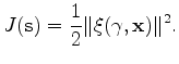
We can now use
as our measure of the residual to minimize, casted as the following objective function:
 |
(7) |
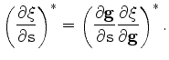
Then, we take the derivative of the objective function with respect to slowness as follows:
 |
(8) |
where 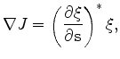 indicates an adjoint. By using the chain rule of differentiation, I relate the derivative of the maximum lag
with respect to
to the derivative of the correlation function with respect to
as follows:
indicates an adjoint. By using the chain rule of differentiation, I relate the derivative of the maximum lag
with respect to
to the derivative of the correlation function with respect to
as follows:
 |
(9) |
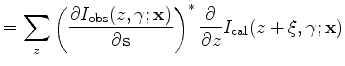
The second partial derivative in equation (9) is just a scalar that balances the energy between surface locations. The first partial derivative with respect to slowness can be calculated using equation (6) as follows:
The first tomographic operator in equation (10) can be computed as I described in equation (4). However, the second tomographic operator depends on how
is computed. If a fixed-reflectivity model is used, such as well data, and only the background slowness is updated, then this derivative will be very small and could be ignored, since changing the slowness updates does not change the reflectivity estimate. On the other hand, if we allow the modeling reflectivity to change location, i.e. we update the reflectivity model as we iterate, then this operator could have a significant component. However, evaluating this operator is much more expensive than the first tomographic operator, since it is a cascade of three operators. Therefore, I will assume that the first tomographic operator is sufficient and ignore the second term.
|
|
|
|
| Correlation-based wave-equation migration velocity analysis | |
|
Next: Synthetic Examples
Up: Almomin: WEMVA
Previous: Introduction
2011-05-24