Model-building with image segmentation and fast image updates

Segmentation process

Under ideal cirmucmstances, automated segmentation using the PRC method can provide a quick and accurate interpretation of regions within a seismic image. For example, the image in Figure 1(a) is a perfect-velocity migration of data from the Sigsbee synthetic model. In the corresponding segmentation result (Figure 1(b)), the salt body is delineated clearly and accurately. Unfortunately, perfect velocity models are non-existent in the real world. Instead, a common approach to building a velocity model in areas dominated by complex salt geology is to pick the top salt after migration with a sediment-flood velocity model, and then pick the base of salt after migration with the resulting salt-flood velocity model (Mosher et al., 2007). It is clear from Figure 2(a), a sediment-flood migration zoomed in to the left half of the salt body, that the salt boundary of a sediment-flood image is not likely to be imaged as well as the perfect-velocity example in Figure 1(a). The resulting segmentation of the image into above- and below-salt regions (Figure 2(b)) is therefore not as accurate.

zig-sfimg,zig-largesfseg2
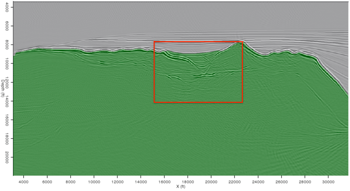
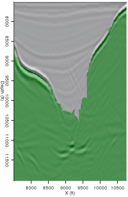
Figure 2. Sediment-flood migration (a), and corresponding segmentation result (b). The segmentation algorithm performs poorly within the area indicated on (b).

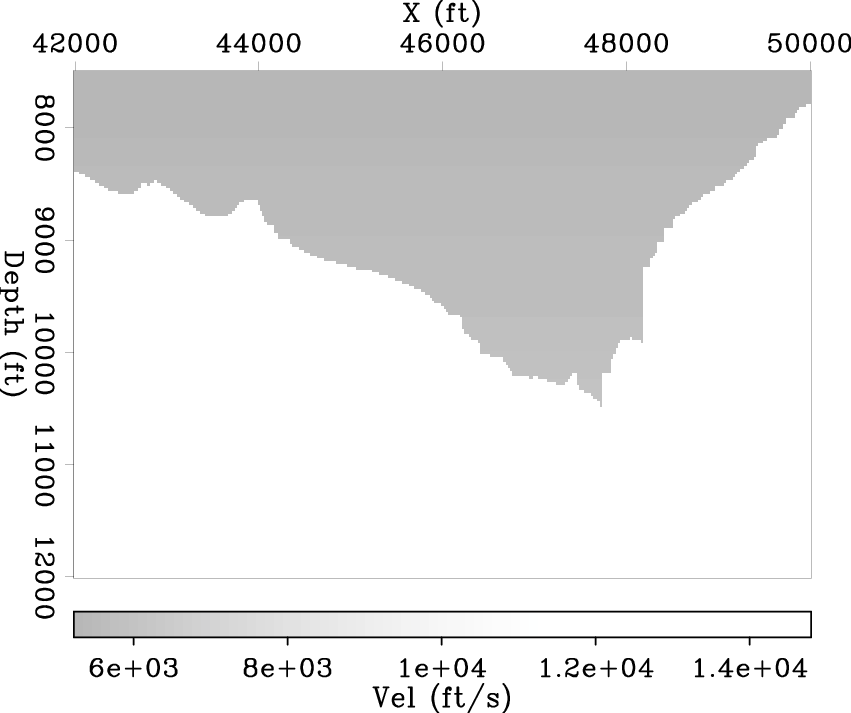
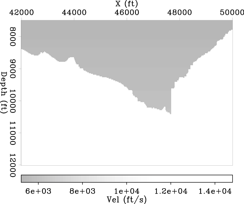
Since the major source of inaccuracy in the Figure 2(b) result is within the salt canyon indicated on the figure, we can restrict our analysis to that region. By setting a smaller minimum segment size, the user can be much more selective about what regions to include as salt. Figures 3(a) and 3(b) display two possible salt interpretations generated by the automatic PRC algorithm for the region in question. In Figure 3(b), an extra segment (indicated by the arrow) has been included in the salt. By replacing segments interpreted as salt with salt velocities on the original sediment flood velocity model, two different velocity models can also be created (Figures 4(a) and 4(b)).

zig-canyonseg1,zig-canyonseg2a
Figure 3. Two possible salt interpretations provided by the segmentation algorithm. In (b), an extra segment (indicated by the arrow) has been included in the salt.

velstitch1,velstitch2
Figure 4. Salt-flood velocity models corresponding to the interpretations in Figures 3(a) and 3(b). The models were created from a sediment-flood velocity model by assigning salt velocities below the interpreted salt boundary.

Model-building with image segmentation and fast image updates