Interpreter input for seismic image segmentation

Three dimensions

While the PRC algorithm suffers from the same leakage problem in 3D (Figure 5(a)) seen in the 2D example, the same solution cannot be applied. Because segments are much larger in 3D, amplitude changes on a single 2D section are not significant enough to alter 3D segmentation results. Instead, we must ``project'' an interpreter's manual picks on an inline section, like those seen in Figure 5(b), into the third (crossline) dimension. If we make the assumption that the dip of the salt flank does not fluctuate by more than two pixels per slice in the crossline direction, we can construct a square pyramid (Figure 6) in the crossline direction with sides of length $2h$ , where $h$ is the number of crossline samples between the base of the pyramid and its apex, which is the manually interpreted point $P$ . Now, the new amplitude value for any pixel $Q$ that falls within the pyramid is

$$A^Q_{\mathrm{new}}=A^Q_{\mathrm{orig}} + \frac{A_0}{\vert\vert PQ\vert\vert},$$ (2)

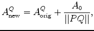
where $A_0$ is the amplitude value at point $P$ as determined by equation (1), and $\vert\vert PQ\vert\vert$ is the distance between the two points. As seen in Figure 7(b), the interpreter's picks now influence amplitude values in all three directions, but the magnitude of that influence decays with distance from the manual picks. Accordingly, the updated 3D segmentation result in Figure 8 is improved throughout the image cube, and not just on the two inline sections where manual picks were provided. For example, Figure 9 shows image slices far away from the two crosslines for which manual interpretations were supplied. In Figures 10(a) and 10(b), the effects of the 3D interpreter input procedure on the envelope volumes are apparent. Figures 11(a) and 11(b) compare the original and interpreter-guided segmentation results for this location, demonstrating that the 3D segmentation results can improve dramatically even far away from any manual pick locations.

o3d-far
Figure 9. Slices from the 3D image cube far away from any interpreter-supplied salt picks.

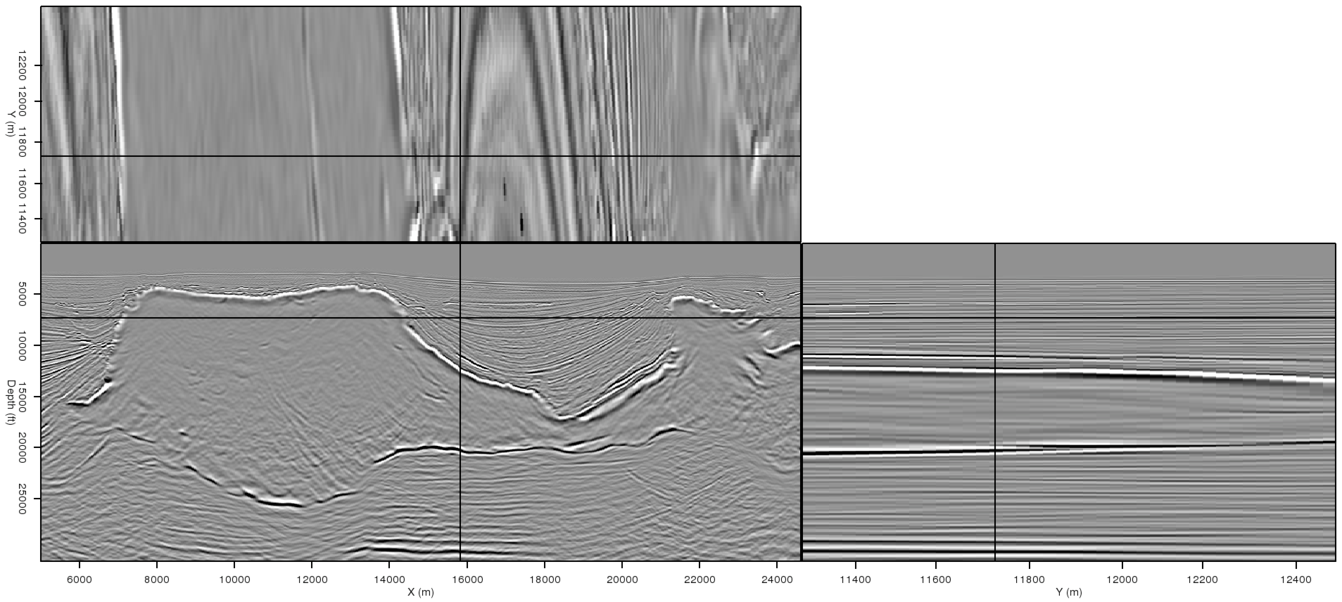
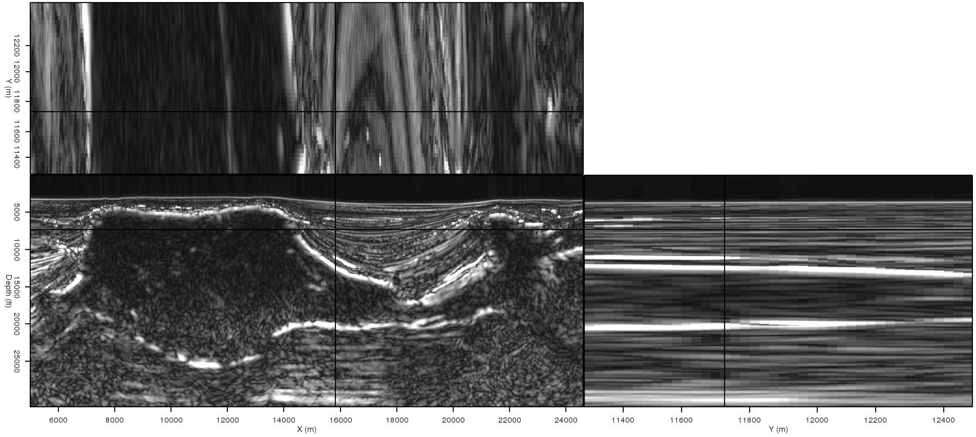
o3d-env-orig-far,o3d-env-new-far
Figure 10. Envelope volumes at the position of the image slices seen in Figure 9, (a) before and (b) after incorporating interpreter input from a distant location. In (b), continuity of the salt boundary is improved, allowing a more accurate segmentation result.

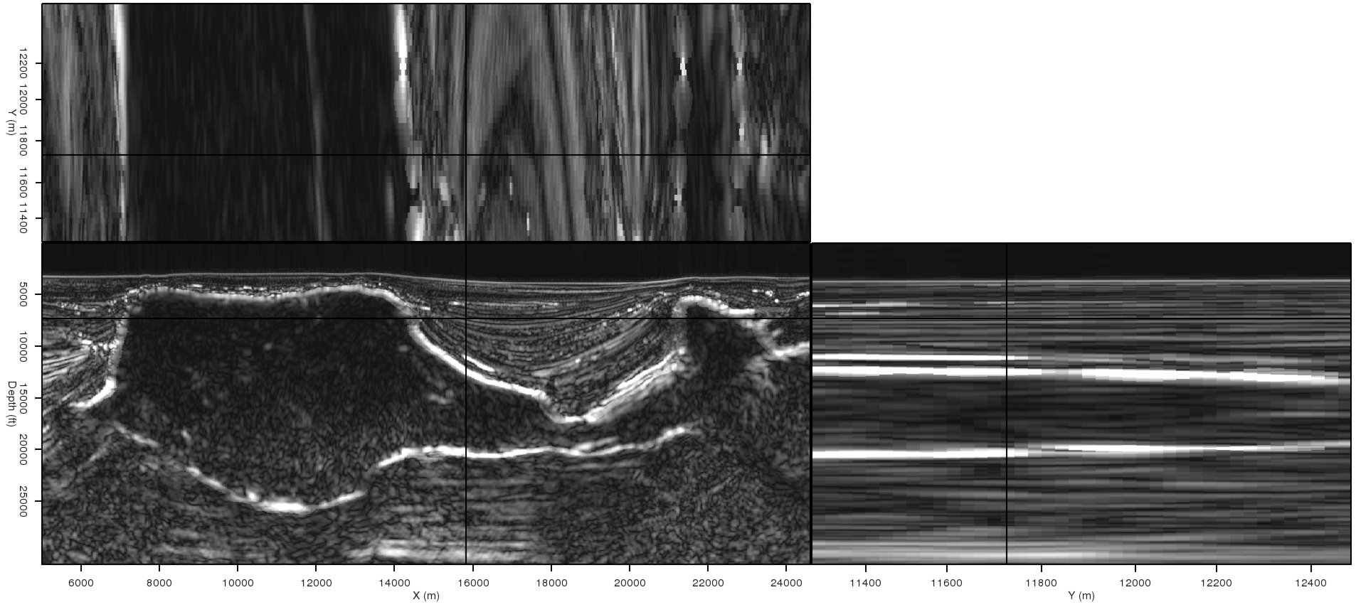
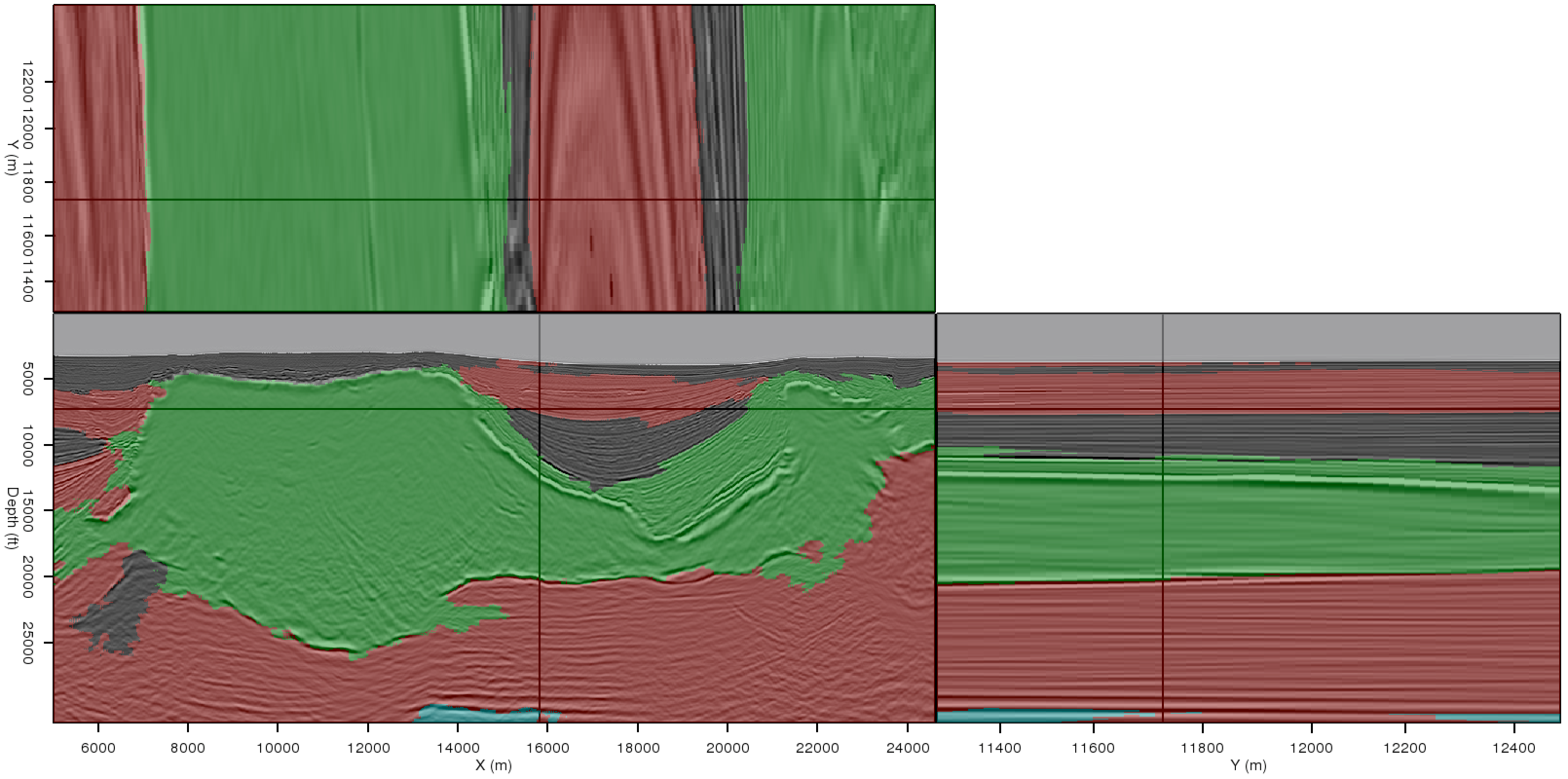
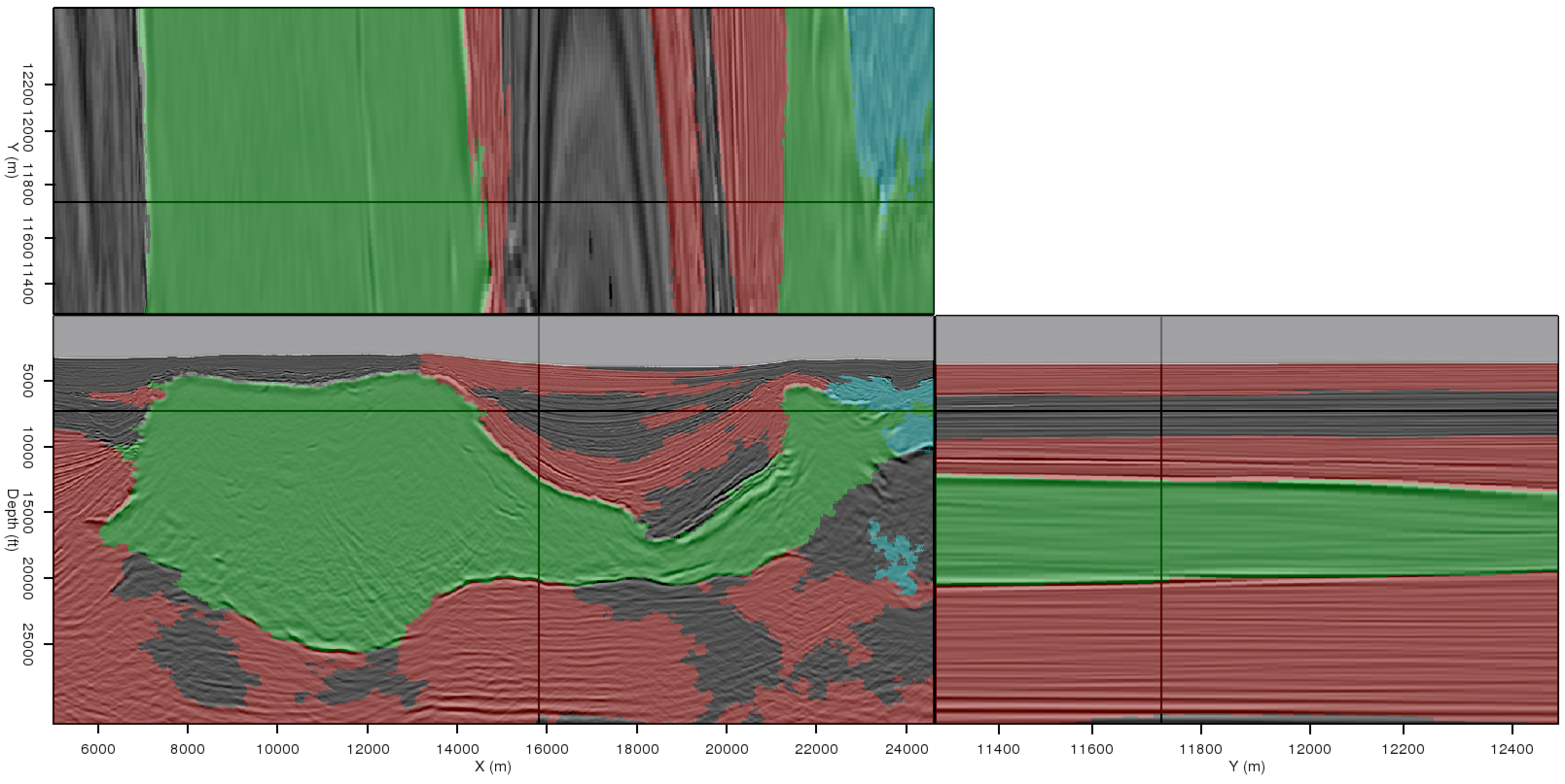
3d-origseg-far,3d-newseg-far
Figure 11. A comparison of segmentation results (a) without using interpreter input, and (b) after incorporating information from the picks in Figure 5(b). Even though the data slices shown here are far from the location of the manual picks, the strategy of spreading information from 2D picks into the third dimension allows for a much more accurate result in (b).

Interpreter input for seismic image segmentation