|
|
|
|
Target-oriented wavefield tomography: A field data example |
Figure 2 shows the initial velocity model for the extracted 2-D line.
Velocities above the target (outlined by a black box) and the salt interpretation are assumed to be accurate.
The goal is to invert for subsalt velocities inside the target region. The initial velocities inside the box are set to
be ![]() .
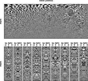
The initial image and subsurface-offset-domain common-image gathers (SODCIGs)
obtained using the original data and the initial velocity model is shown in
Figure 3. The amplitudes of the initial image have been balanced
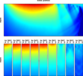
by the diagonal of the Hessian (Figure 4) according to equation 3 to
compensate for uneven subsalt illumination and remove the influence of the original data acquisition geometry.
Note the unfocused SODCIGs due to velocity errors.
.
The initial image and subsurface-offset-domain common-image gathers (SODCIGs)
obtained using the original data and the initial velocity model is shown in
Figure 3. The amplitudes of the initial image have been balanced
by the diagonal of the Hessian (Figure 4) according to equation 3 to
compensate for uneven subsalt illumination and remove the influence of the original data acquisition geometry.
Note the unfocused SODCIGs due to velocity errors.
Then we use the target image (Figure 3) and the Born modeling described in the previous section to generate
![]() plane-wave-source gathers at the top of the target region,
where the take-off angle is from
plane-wave-source gathers at the top of the target region,
where the take-off angle is from
![]() to
to
![]() . The same starting velocity model that was used for migration
(Figure 2) has been used for modeling,
and the new data set is collected just above the target region. We only model Born wavefields up to
. The same starting velocity model that was used for migration
(Figure 2) has been used for modeling,
and the new data set is collected just above the target region. We only model Born wavefields up to ![]() Hz.
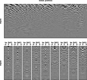
Figure 5 shows the image migrated using the new data set and the initial velocity
(Figure 2).
Note the same kinematics shown in Figures 3 and 5.
This suggests that the velocity information has been successfully preserved using the new data set, which is substantially smaller compared
to the original one.
Hz.
Figure 5 shows the image migrated using the new data set and the initial velocity
(Figure 2).
Note the same kinematics shown in Figures 3 and 5.
This suggests that the velocity information has been successfully preserved using the new data set, which is substantially smaller compared
to the original one.
We minimize the objective function ![]() (equation 7) using a nonlinear conjugate gradient solver.
Figure 6 shows the inverted velocity model after
(equation 7) using a nonlinear conjugate gradient solver.
Figure 6 shows the inverted velocity model after ![]() iterations.
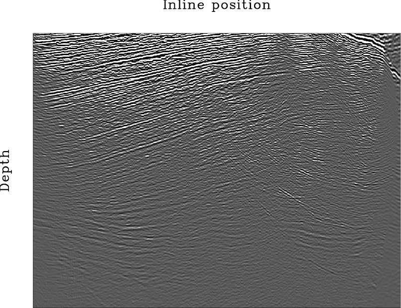
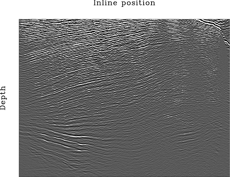
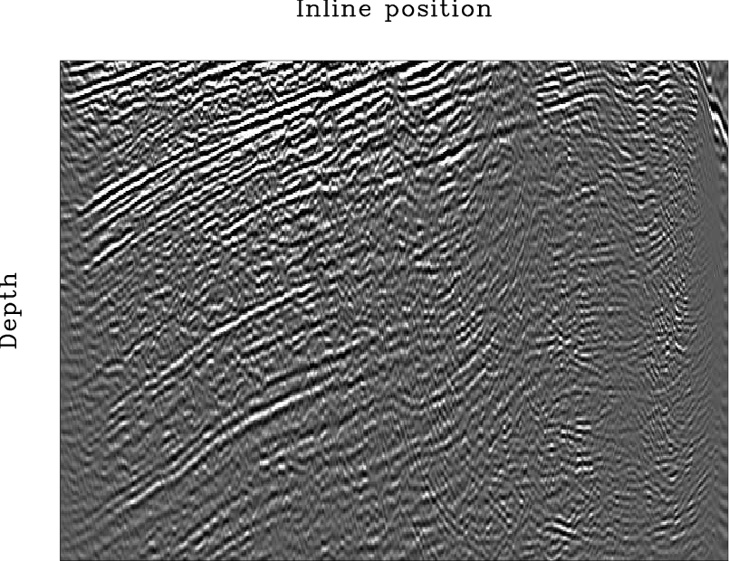
We then migrate the original data set using the inverted model and compare the result with that obtained
using the initial velocity model.
Figures 7,
8 and
9
compare the
stacked section (zero-subsurface-offset image) using the initial and updated velocities.
The image obtained using the inverted velocity model
shows improved continuities, better focusing and higher signal to noise ratio.
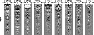
The angle domain common image gathers (ADCIGs) migrated using the inverted velocity mode (Figure 10(b))
are also flatter comparing to those obtained using the initial velocity model (Figure 10(a)).
iterations.
We then migrate the original data set using the inverted model and compare the result with that obtained
using the initial velocity model.
Figures 7,
8 and
9
compare the
stacked section (zero-subsurface-offset image) using the initial and updated velocities.
The image obtained using the inverted velocity model
shows improved continuities, better focusing and higher signal to noise ratio.
The angle domain common image gathers (ADCIGs) migrated using the inverted velocity mode (Figure 10(b))
are also flatter comparing to those obtained using the initial velocity model (Figure 10(a)).

|
|---|
|
wemva-bpgom2d-bvel
Figure 2. The initial velocity model for the selected 2-D line. The black box outlined area is the target region for velocity analysis. Velocities outside the region are assumed to be accurate. [NR] |
|
|
|
|---|
|
wemva-bpgom2d-bimg-target-odcig
Figure 3. Initial target image and gathers obtained using the original data and the initial velocity shown in Figure 2. Top panel shows the stacked image (zero subsurface offset); bottom panel shows the SODCIGs for different horizontal locations. [NR] |
|
|
|
|---|
|
wemva-bpgom2d-bhes-target-odcig
Figure 4. The diagonal of Hessian for the target region. View descriptions are the same as in Figure 3. [NR] |
|
|
|
|---|
|
wemva-bpgom2d-bimg-odcig-born-planes
Figure 5. Image and gathers obtained using the new data set and the initial velocity (Figure 2). View descriptions are the same as in Figure 3. [NR] |
|
|

|
|---|
|
wemva-bpgom2d-invt-vmod
Figure 6. The inverted velocity model after |
|
|
|
|---|
|
wemva-bpgom2d-bimg-stack-raw-slides,wemva-bpgom2d-invt-stack-raw-slides
Figure 7. Stacked images (zero-subsurface-offset images) obtained using (a) the initial velocity model and (b) the inverted velocity model. The original data set is used for migration. [NR] |
|
|

|
|---|
|
wemva-bpgom2d-bimg-stack-raw-zoom1,wemva-bpgom2d-invt-stack-raw-zoom1
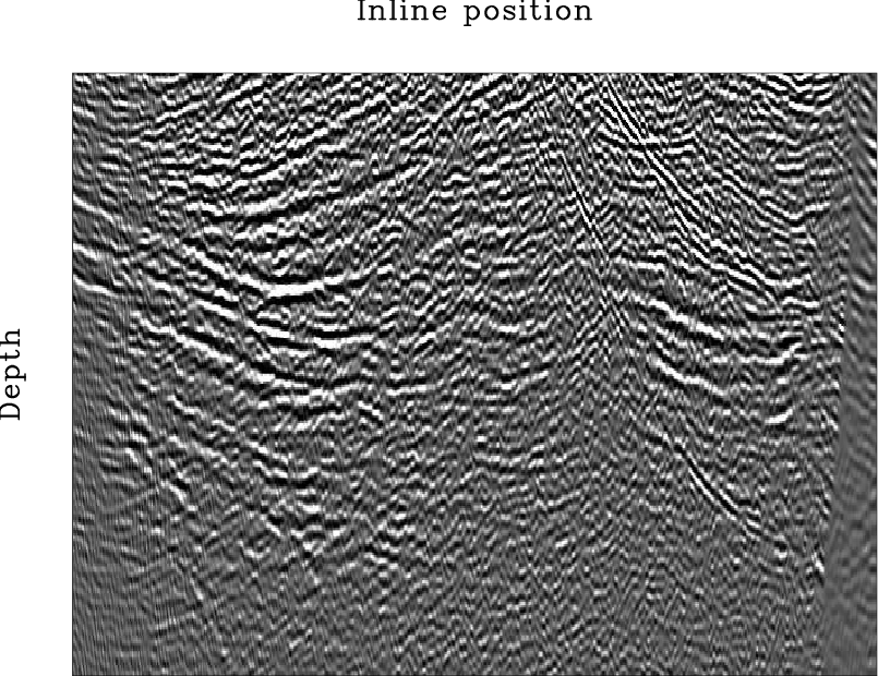
Figure 8. A close-up view of the upper section in Figure 7. (a) is obtained using the initial velocity model and (b) is obtained using the inverted velocity model. [NR] |
|
|
|
|---|
|
wemva-bpgom2d-bimg-stack-raw-zoom2,wemva-bpgom2d-invt-stack-raw-zoom2
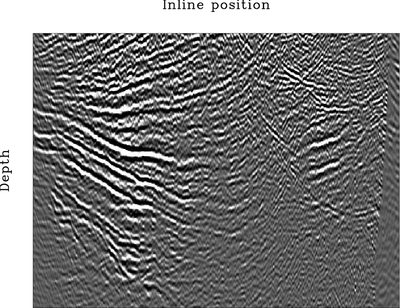
Figure 9. A close-up view of the lower section in Figure 7. (a) is obtained using the initial velocity model and (b) is obtained using the inverted velocity model. [NR] |
|
|

|
|---|
|
wemva-bpgom2d-bimg-adcig-slides,wemva-bpgom2d-imag-invt-adcig-slides
Figure 10. Angle-domain common-image gathers obtained using (a) the initial velocity model and (b) the inverted velocity model. The original data set is used for migration. [NR] |
|
|
|
|
|
|
Target-oriented wavefield tomography: A field data example |