Implementing implicit finite-difference in the time-space domain using spectral factorization and helical deconvolution

Effect of floating point precision

As a result of the tests shown in the previous section, I concluded that the reason for the unstable propagation at large time step sizes had to do with the spectral factorization, and not with the finite-difference approximation. One of the characteristics of the filter coefficients produced by the spectral factorization algorithm I used (SEPlib module wilson) is that they are very small. The smaller ones can reach $10^{-20}$ . Biondi and Clapp (pers. comm., 2010) suggested that I attempt to use double precision variables instead of single precision, in order to see whether the precision of the representation of the filter coefficients is indeed an issue. Ronen (pers. comm., 2010) also suggested trying to do the opposite - reduce the precision and see whether that would have a degrading effect on the propagation.

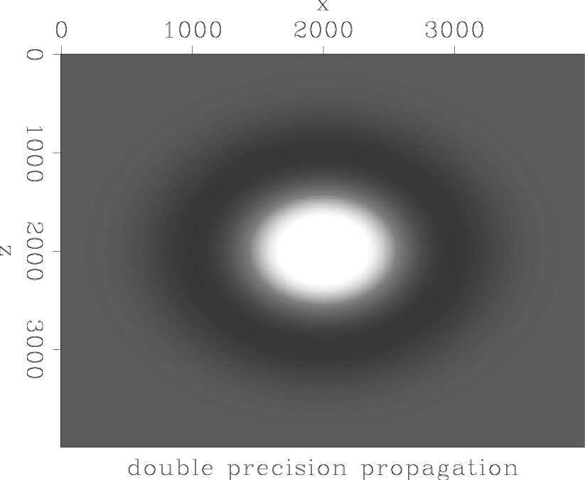
To achieve double precision, both the spectral factorization algorithm and the helical deconvolution module had to be rewritten to include double precision variables. The wavefield itself was also composed of double precision variables. Furthermore, I used a 4th order in space, 2nd order in time approximation for this test. Figures 7(a)-7(d) show the comparison between propagation with single precision (left) and double precision (right). For the top Figures I used $\epsilon = 0$ , and for the bottom ones $\epsilon = 0.01$ . The time step $\Delta t$ was $10 ms$ for all Figures. The results for single and double precision are identical for this time step, and from other tests with many different time step sizes I can say that the behaviour is always identical, and so is the response to varying value of $\epsilon$ . The similarity in the wavefield values extends to the statistics of the wavefields - the mean, average, RMS and min/max values are nearly identical as well. In summary - I could not find a set of parameters for which propagation with double precision variables is better (or at all different) than propagation with single precision.

The next step was to attempt to reduce the precision of the spectrally factorized coefficients one decimal point at a time, and see when propagation with a certain set of parameters is destroyed as a result of this loss of precision. This should give an indication as to how important the floating point precision actually is for stable propagation. The precision reduction was done by running the regular wilson spectral factorization subroutine, and then reducing precision by the following two lines of code:
noindent IntFilter = CutFactor * FloatFilter
FloatFilter = IntFilter / CutFactor

CutFactor is a power of 10. Multiplying by this factor and then casting to integer effectiveley removes decimal precision from the filter coefficients. Example:
10000 * 1.23456 = 12345
12345 / 10000 = 1.2345

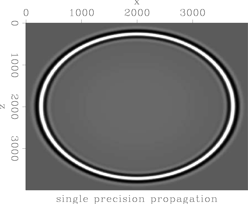
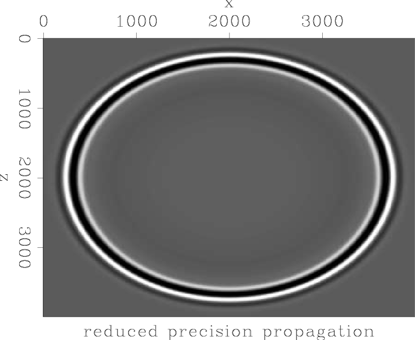
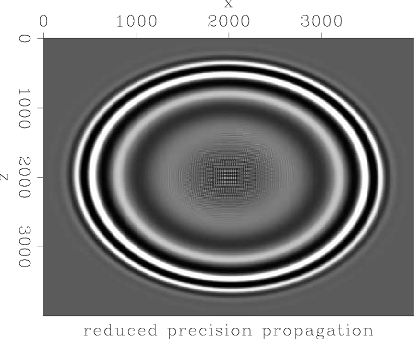
The purpose of this test was to see how many decimal precision digits can be removed from the filter coefficients before wavefield propagation using those coefficients is altered, in comparison to propagation with standard floating point precision. Results can be seen in Figures 8(a)-8(c). On the left is the result of propagation with single precision coefficients, with parameters which have shown stability ( $\Delta t = 5ms, \epsilon = 0$ ). The center Figure shows propagation with coefficients which have had their precision truncated to 3 decimal points only. The wavefield exhibits a phase shift in comparison to the single precision wavefield, and yet it remains stable. Only when precision is truncated to 2 decimal points (right) is propagation severely affected.
The wavefields in Figures 7(a)-7(d) and 8(a)-8(c) were generated using factorization of the finite-difference weights of the 4th spatial order approximation (A-1). The values of these weights when using the specific set of propagation parameters were:
$U_0 = 1.3125,\ \ \ \ \ \ U_1 = -8.3333343E-02, \ \ \ \ \ \ U_2 = 5.2083340E-03$ .

Since $\Delta x = \Delta z$ , the weights are identical for both dimensions. These weights are fed to the spectral factorization routine, which is supposed to produce a causal set of filter coefficients, such that their cross-correlation will reproduce the finite-difference weights (Claerbout, 1997). This suggests that one way of testing the sensitivity of propagation to the floating point precision of the filter coefficients is to correlate the filter coefficients and compare the result to the finite-difference weights.

I used 21 filter coefficients to produce Figures 8(a)-8(c). For single precision propagation, the values of the correlation of the filter coefficients were (Only the first four values of the correlation are displayed. The rest are in A-2 to A-4):

$$\begin{array}{cccc} 1.312500 & -8.3333343E-02 & 5.2083335E-03 & 2.9154580E-12\end{array}$$

For the propagation where precision was reduced to 3 decimal points only, the correlation was:

$$\begin{array}{cccc} 1.312500 & -8.3329208E-02 & 5.2077500E-03 & 0.0000000E+00\end{array}$$

For the propagation where precision was reduced to 2 decimal points only, the correlation was:

$$\begin{array}{cccc} 1.312500 & -7.8187048E-02 & 0.0000000E+00 & 0.0000000E+00\end{array}$$

Note that the correlation products are arranged in order of lags, so that the first coefficient corresponds to the central finite-difference weight $U_0$ , the second to $U_1$ , and the third to $U_2$ . Note also that only after reducing precision to the 2nd decimal point, the weight $U_2$ is effectively erased, and the weight $U_1$ is considerably altered.

This comparison proves that the wavefield divergence shown in the previous sections is not the result of inadequate representation of the filter coefficient's floating point values when using single precision. If it were, then propagation with reduced precision would not have been possible. However, this result raises another question: If propagation is stable with so little precision, how come a small value of $\epsilon$ added to the central finite-difference weight (and by that also to the zero-lag filter coefficient) causes the wavefield to stabilize, when the effect that this slight addition has on the filter's correlation is so much less pronounced than the precision reduction?

double-vs-single1-a,double-vs-single1-b,double-vs-single1-c,double-vs-single1-d
Figure 7. 2D helical implicit finite-difference using single (left) and double (right) precision. Velocity = $1000 m/s$ . Wavefields are after 2 seconds of propagation. Source is a Ricker wavelet with central frequency = $12.5 Hz$ . The time step size is $\Delta t = 10 ms$ . $\epsilon = 0$ for the top Figures, and $\epsilon = 0.01$ for the bottom Figures. $\Delta x = \Delta z = 10 m$ .[ER]

single-vs-half-a,single-vs-half-b,single-vs-half-c
Figure 8. 2D helical implicit finite-difference using single precision (left), precision reduced to 3 decimal points (center), and precision reduced to 2 decimal points (right). Velocity = $1000 m/s$ , $\Delta t = 5 ms$ , $\epsilon = 0$ , $\Delta x = \Delta z = 10 m$ .[ER]

Implementing implicit finite-difference in the time-space domain using spectral factorization and helical deconvolution