|
|
|
|
Implementing implicit finite-difference in the time-space domain using spectral factorization and helical deconvolution |
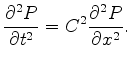
The two-way acoustic wave equation in one dimension reads:
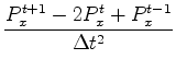
The central implicit finite-difference approximation I used for the propagation tests was 2nd order in time and 2nd order in space:
where ![]() is the pressure wavefield,
is the pressure wavefield, ![]() and
and ![]() are the time and space coordinate indices, and
are the time and space coordinate indices, and ![]() and
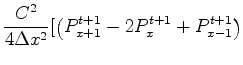
and ![]() are the temporal and spatial step sizes. Note that this approximation is based on the Crank-Nicolson method, and so the spatial derivative is balanced between the three time steps:
are the temporal and spatial step sizes. Note that this approximation is based on the Crank-Nicolson method, and so the spatial derivative is balanced between the three time steps: ![]() ,
, ![]() , and
, and ![]() , where the central time index
, where the central time index ![]() has twice the weight of the other two time indices.
has twice the weight of the other two time indices.
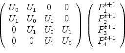
In order to propagate the wavefield, the pressure values at time ![]() must be equated to the values at times
must be equated to the values at times ![]() and
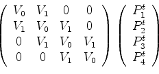
and ![]() . The linear system which must then be solved has the form:
. The linear system which must then be solved has the form:
For simplicity, we can combine all the constants into one:
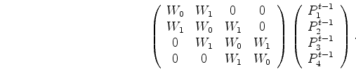 .
The matrix coefficients in equation 3 (the finite-difference weights) are then:
.
The matrix coefficients in equation 3 (the finite-difference weights) are then:
![]()
![]()
![]()
In shorter notation, equation 3 reads:
The solution of this linear system is:
To solve this system, we must perform polynomial division. The system is tridiagonal (and easily solvable) only for one dimension. For multiple dimensions, matrix ![]() is block diagonal. Additional non-zero elements appear at a certain offset from the diagonal, making the solution process more complicated. However, using spectral factorization, the finite-difference weights of matrix
is block diagonal. Additional non-zero elements appear at a certain offset from the diagonal, making the solution process more complicated. However, using spectral factorization, the finite-difference weights of matrix ![]() (which pertain to time
(which pertain to time ![]() ) can be factorized into a set of causal filter coefficients
) can be factorized into a set of causal filter coefficients ![]() and its time reverse
and its time reverse ![]() . Using the helical approach to deconvolution, equation 5 can be recast as:
. Using the helical approach to deconvolution, equation 5 can be recast as:
Polynomial division is comparable to deconvolution. This means that the polynomial division in equation 5 can be achieved by a set of two deconvolutions of the data by the spectrally factorized coefficients ![]() of matrix
of matrix ![]() . One deconvolution is done along the data in the reverse direction (application of the adjoint of the filter):
. One deconvolution is done along the data in the reverse direction (application of the adjoint of the filter):
 is the time reversed filter coefficients of
I used the SEPlib module polydiv, which uses the helical coordinates to perform the deconvolutions (the polynomial division) in equations 8 and 9.
The wavefield propogation is done by the following sequence:
 .
.
Steps 2 - 6 are repeated for each time step. The inputs of the spectral factorization are the finite-difference weights of the matrix ![]() (in Eq. 3), and the outputs are coefficients of a minumum phase filter
(in Eq. 3), and the outputs are coefficients of a minumum phase filter ![]() . Since I used a constant velocity in all propagation tests, the finite-difference weights are constant, and the filter is stationary.
. Since I used a constant velocity in all propagation tests, the finite-difference weights are constant, and the filter is stationary.
|
|
|
|
Implementing implicit finite-difference in the time-space domain using spectral factorization and helical deconvolution |