|
|
|
|
Implementing implicit finite-difference in the time-space domain using spectral factorization and helical deconvolution |
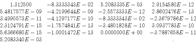
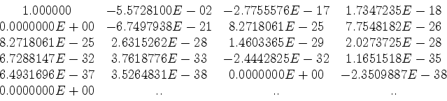
The correlation of the 21 filter coefficients used to create Figure 8(a) for single precision propagation was (I apologize for having the temerity to show raw numbers, but I couldn't find a suitable graphic representation):
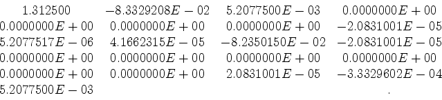
For propagation where precision was reduced to 3 decimal points only, the correlation was:
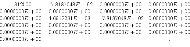
For propagation where precision was reduced to 2 decimal points only, the correlation was:
The correlation products are arranged in order of lags. Since the finite-difference operator is two dimensional, the weights for ![]() and
and ![]() reappear at lags corresponding to the wrap-around of the 1D filter around the edges of the 2D grid (in helical coordinates). Therefore the 11th coefficient is equal to the 2nd coefficient, and the 21st is equal to the 3rd.
reappear at lags corresponding to the wrap-around of the 1D filter around the edges of the 2D grid (in helical coordinates). Therefore the 11th coefficient is equal to the 2nd coefficient, and the 21st is equal to the 3rd.
The 50 filter coefficients used to produce Figure 9:
After lag 20, the coefficients were all zeros. The correlation of these coefficients was:
|
|
|
|
Implementing implicit finite-difference in the time-space domain using spectral factorization and helical deconvolution |
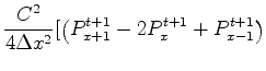
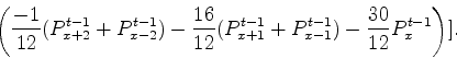
![$\displaystyle \left( \frac{-1}{12}(P^{t-1}_{x+2} + P^{t-1}_{x-2}) - \frac{16}{12}(P^{t-1}_{x+1} + P^{t-1}_{x-1}) - \frac{30}{12}P^{t-1}_x \right)
].$](img81.png)