On the separation of simultaneous-source data by inversion

Example 1: Separation of complex data sets

In this example, we consider data from a complex 2D salt model (Figure 1(a)). The simultaneous-source data comprise $330$ shot gathers from two sources separated by ${2400}$ m (Figure 2). This example represents the case where a front seismic vessel is pulling the streamer, and a second boat shoots from the end of the streamer cable-- with both sources moving from left to right over the model in Figure 1(a). Note the randomness of data corresponding to the unaligned source in the common-offset plane. The single-source records are shown in Figure 3. The separated data sets recovered by $l_{2}$ (conjugate-gradient) inversion are shown in Figure 4. Comparing these results to the single-source data (Figure 3), we see that there are numerous crosstalk artifacts in each of the two sources. Separation results obtained by sparse inversion of the data without and with regularization by directional Laplacians are shown in Figures 5 and 6, respectively. Note that in both inversion results, the data are well separated into the component shot records. The residual artifacts present in the unconstrained sparse-inversion results (Figure 5) have been attenuated by regularization (Figure 6). Dips estimated from the unconstrained results (Figure 5) and used to obtain the dip-constrained results (Figure 6) are shown in Figure 7.

2s5-or-1
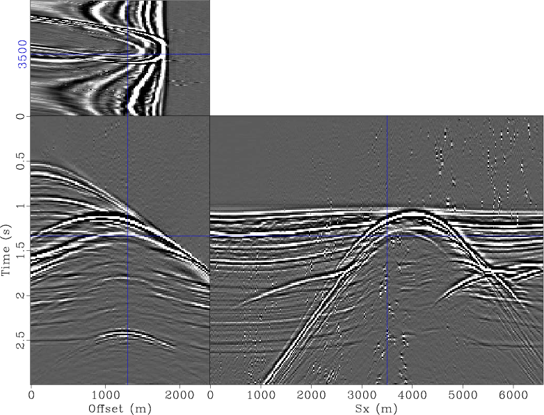
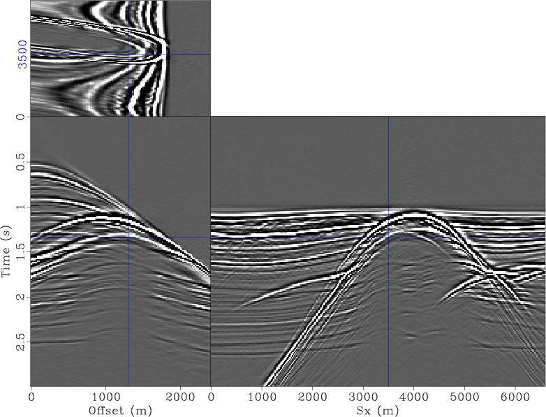
Figure 2. Simultaneous-source data comprising shot-records from two end-on sources (S1 and S2) over the model in Figure 1(a). In this and subsequent figures, the second dimension is offset, and the third dimension is shot position. Note that along the common-offset axis, because the shot times have been referenced to source S1, data corresponding to this source are aligned, whereas those corresponding to S2 are not aligned.

2s5-1,2s5-2
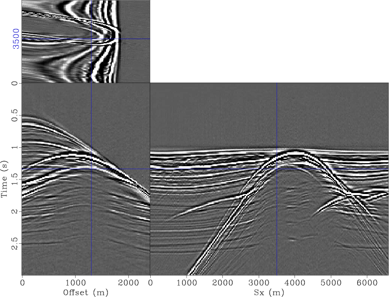
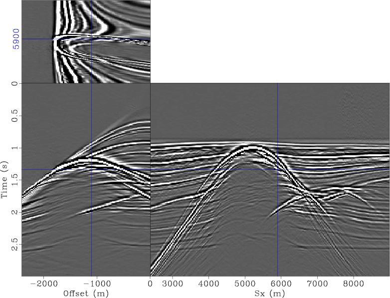
Figure 3. Single-source data that would have been recorded by (a) source 1 and (b) source 2 over the model in Figure 1(a). These two shot records are the components of the data shown in Figure 2.

2s5-l2-1,2s5-l2-2
Figure 4. Shot gathers recovered by unconstrained $l_{2}$ inversion for (a) source 1 and (b) source 2. Note that the two data sets are not well separated, as several events which do not exist in the single-source data (Figure 3) are present.

2s5-hb-1,2s5-hb-2
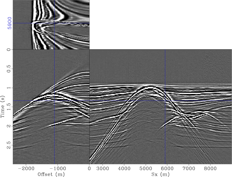
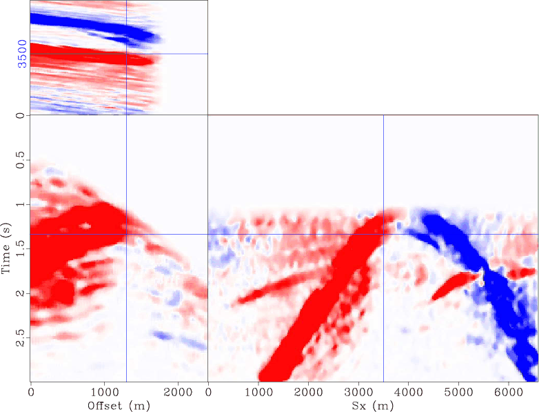
Figure 5. Shot gathers recovered by unconstrained sparse inversion for (a) source 1 and (b) source 2. Note that the two data sets are well separated and are comparable to the original data (Figure 3).

2s5-reg-1,2s5-reg-2
Figure 6. Shot gathers recovered by dip-constrained sparse inversion for (a) source 1 and (b) source 2. Note that with regularization the residual artifacts present in the unconstrained example (Figure 5) have been attenuated.

2s5-dip-1,2s5-dip-2
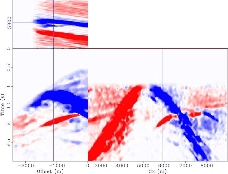
Figure 7. Local dips (common-offset components) for (a) source 1 and (b) source 2, obtained from the unconstrained sparse inversion (Figure 5) and used in the dip-constrained sparse inversion to obtain the results in Figure 6.

On the separation of simultaneous-source data by inversion