|
|
|
|
Angle-domain illumination gathers by wave-equation-based methods |
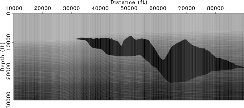
We test our methods on the Sigsbee2A model, where the complex salt body and limited acquisition geometry result in uneven subsurface illumination
below the salt. The velocity field shown in Figure 14 is used for computing various angle-domain reflectivity images and illumination.
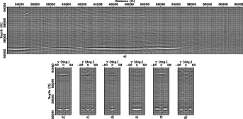
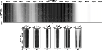
Figure 15 shows the scattering-angle-domain reflectivity image. Note the holes in the scattering-angle gathers
(Figures 15(b)-(g)) caused by uneven illumination. This phenomenon should conform with the angle-domain illumination.
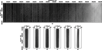
As expected, the scattering-angle-domain illumination (Figure 16)
fails to accurately predict the illumination pattern for planar reflectors, e.g., the horizontal reflector at depth ![]() ft,
although it is very accurate for the point scatterers locatd at depth
ft,
although it is very accurate for the point scatterers locatd at depth ![]() ft.
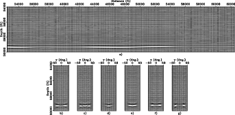
We further decompose the image and illumination into dip-dependent scattering-angle domain. The illumination pattern (Figure 18)
now conforms very well
with the image of the planar reflectors (Figure 17) as well as the reflectors that have a zero dip in Figure 15.
ft.
We further decompose the image and illumination into dip-dependent scattering-angle domain. The illumination pattern (Figure 18)
now conforms very well
with the image of the planar reflectors (Figure 17) as well as the reflectors that have a zero dip in Figure 15.
|
|---|
|
sigsb2a-vmig
Figure 14. Sigsbee2A velocity model used for migration and illumination computation. [ER] |
|
|
|
|---|
|
sigsb2a-imag-adcig
Figure 15. Scattering-angle-domain reflectivity image for the Sigsbee2A model. Panel (a) shows the image with scattering angle |
|
|
|
|---|
|
sigsb2a-hess-adcig
Figure 16. Scattering-angle-domain illumination for the Sigsbee2A model. View descriptions are the same as Figure 15. [CR] |
|
|
|
|---|
|
sigsb2a-imag-adcig-dip
Figure 17. Dip-dependent scattering-angle-domain reflectivity image for the Sigsbee2A model. Panel (a) shows the image with scattering angle |
|
|
|
|---|
|
sigsb2a-hess-adcig-dip
Figure 18. Scattering-angle-domain illumination for the Sigsbee2A model. View descriptions are the same as Figure 17. [CR] |
|
|
|
|
|
|
Angle-domain illumination gathers by wave-equation-based methods |