|
|
|
|
Angle-domain illumination gathers by wave-equation-based methods |
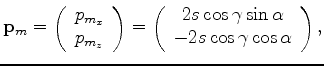
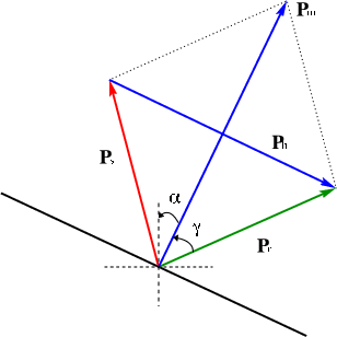
In a locally constant velocity medium (Figure 1),
the midpoint ray parameter ![]() and the subsurface offset ray parameter
and the subsurface offset ray parameter ![]() can be expressed as follows:
can be expressed as follows:
| (7) | |||
| (8) |
 is the slowness at the reflection point.
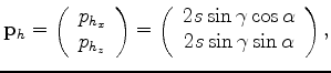
Dividing
is the slowness at the reflection point.
Dividing 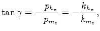 and
and
|
local-phase-relation
Figure 1. Geometric relations between ray vectors at a reflection point in a locally constant velocity medium. [NR] |
|
|---|---|
|
|
We obtain the scattering-angle-domain Hessian by correlating the sensitivity kernels
![]() as follows:
as follows:
 and
and

 ,
,
As a simple example,
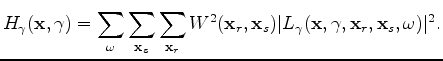
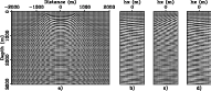
Figures 3 shows the real part of the scattering-angle-domain sensitivity kernel, converted from
its subsurface-offset-domain counterpart (Figure 2).
The results are obtained by using a constant velocity model (![]() m/s), and only
one source (
m/s), and only
one source (![]() m), one receiver (
m), one receiver (![]() m) and one frequency (
m) and one frequency (![]() Hz) are computed.
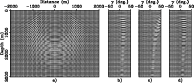
Figure 4 shows
the corresponding single-frequency scatter-angle-domain illumination for the given velocity model and acquisition configuration.
Since there are only one source and one receiver, each subsurface point is illuminated by only one scattering angle.
Hz) are computed.
Figure 4 shows
the corresponding single-frequency scatter-angle-domain illumination for the given velocity model and acquisition configuration.
Since there are only one source and one receiver, each subsurface point is illuminated by only one scattering angle.
The scattering-angle-domain illumination is useful for point scatterers,
it, however, fails to accurately predict the illumination strength for planar reflectors, where the scattered waves have preferred orientations according
to the local dips of the reflectors.
The reason behind this is that the transformation (equation 11) is dip-independent,
the resulting angle-domain illumination implicitly averages over all dip angles
and measures the overall scattering-angle illumination from all dips illuminated, instead of the illumination from one particular dip of
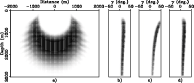
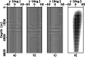
the actual planar reflector. This point is further illustrated by Figures 5 and 6,
where the computed scattering-angle-domain illumination (Figure 6(d)) accurately predicts the illumination
for the point scatterer (Figures 5(c) and 6(c)),
instead of the horizontal (Figures 5(a) and 6(a))
and the
![]() dipping reflectors (Figures 5(b) and 6(b)).
dipping reflectors (Figures 5(b) and 6(b)).
|
|---|
|
const-kernel-odcig-1s1r-1w
Figure 2. The real part of the subsurface-offset-domain sensitivity kernel for a constant velocity model ( |
|
|
|
|---|
|
const-kernel-adcig-1s1r-1w
Figure 3. The real part of the scattering-angle-domain sensitivity kernel after conversion from the subsurface offset domain (Figure 2). Panel (a) shows the sensitivity kernel for a constant scattering angle |
|
|
|
|---|
|
const-hess-adcig-1s1r-1w
Figure 4. The single-frequency scattering-angle-domain illumination obtained using the sensitivity kernel shown in Figure 3. Panel (a) shows the illumination for scattering angle |
|
|
|
|---|
|
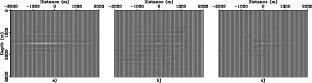
const-imag-stack
Figure 5. Migrated zero-subsurface-offset images (stacked images) for (a) a horizontal reflector, (b) a dipping reflector ( |
|
|
|
const-imag-adcig
Figure 6. The scattering-angle-domain image gathers extracted at spatial location 0 m for (a) the horizontal reflector, (b) the dipping reflector and (c) the point scatterer. Panel (d) shows the scattering-angle-domain illumination gather extracted at the same spatial location. [CR] |
|
|---|---|
|
|
|
|
|
|
Angle-domain illumination gathers by wave-equation-based methods |