|
 |
 |
 | Target-oriented wavefield tomography using demigrated Born data |  |
![[pdf]](icons/pdf.png) |
Next: tomographic inversion results
Up: Tang and Biondi: Image-domain
Previous: Target-oriented Born wavefield modeling
The objective function of image-domain wavefield tomography can be defined as the  norm of either
an image-domain residual field (Shen, 2004; Sava, 2004) or
the negative image-stack power (or image coherence) (Toldi, 1985; Soubaras and Gratacos, 2007) or both (Shen and Symes, 2008).
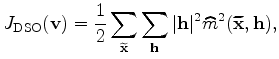
A widely used residual operator is the subsurface-offset-domain differential semblance optimization (DSO) operator,
where the velocity model is optimized by penalizing energy at non-zero subsurface offset, utilizing the fact that
the SODCIGs should be focused at zero subsurface offset if migrated using an accurate velocity model.
The DSO objective function reads (Shen, 2004)
norm of either
an image-domain residual field (Shen, 2004; Sava, 2004) or
the negative image-stack power (or image coherence) (Toldi, 1985; Soubaras and Gratacos, 2007) or both (Shen and Symes, 2008).
A widely used residual operator is the subsurface-offset-domain differential semblance optimization (DSO) operator,
where the velocity model is optimized by penalizing energy at non-zero subsurface offset, utilizing the fact that
the SODCIGs should be focused at zero subsurface offset if migrated using an accurate velocity model.
The DSO objective function reads (Shen, 2004)
 |
|
|
(9) |
where
 is the subsurface-offset-domain image migrated using velocity
  (equation 5)
and the Born-modeled data described in the previous section.
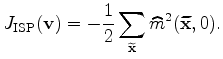
In contrast, minimizing the negative image-stack power (ISP) utilizes the fact
that the stacked image should achieve maximum energy (or focus) when migrated with an accurate velocity (Toldi, 1985; Soubaras and Gratacos, 2007).
Since the zero-subsurface-offset image is the stacked image, the ISP objective function reads
(equation 5)
and the Born-modeled data described in the previous section.
In contrast, minimizing the negative image-stack power (ISP) utilizes the fact
that the stacked image should achieve maximum energy (or focus) when migrated with an accurate velocity (Toldi, 1985; Soubaras and Gratacos, 2007).
Since the zero-subsurface-offset image is the stacked image, the ISP objective function reads
 |
|
|
(10) |
The above two objective functions can also be combined into one single objective function as follows (Shen and Symes, 2008):
 |
|
|
(11) |
where 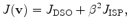 is a constant to trade off these two objective functions.
The gradients can be calculated using the adjoint-state method without explicitly building the sensitivity matrix,
see, e.g. Sava and Vlad (2008); Tang et al. (2008), for implementation details.
The gradient is then used to update the velocity model with a suitable step length chosen by a line-search step.
We iterate this process until an acceptable velocity model is obtained.
is a constant to trade off these two objective functions.
The gradients can be calculated using the adjoint-state method without explicitly building the sensitivity matrix,
see, e.g. Sava and Vlad (2008); Tang et al. (2008), for implementation details.
The gradient is then used to update the velocity model with a suitable step length chosen by a line-search step.
We iterate this process until an acceptable velocity model is obtained.
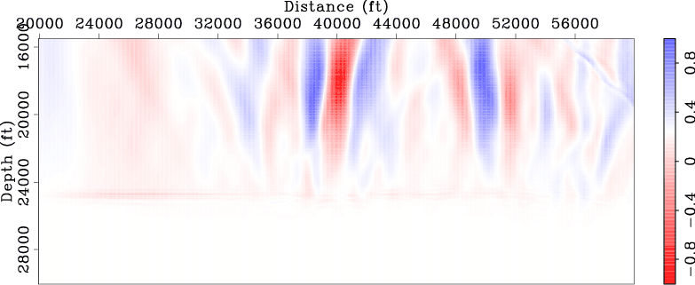
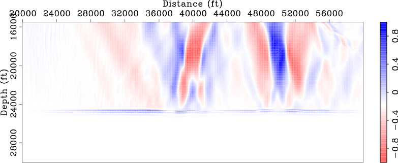
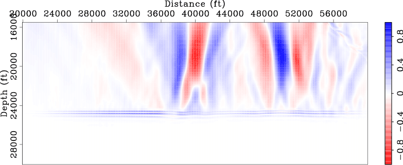
Figures 5 and 6
compare the normalized DSO and ISP gradients
obtained using the original data set with those obtained using the new data set. These gradients are computed using the
starting velocity model (Figure 1(b)).
Note that both DSO and ISP gradients correctly identify those two anomalies
and they also give correct directions for velocity updates. Also note that the gradients obtained using the new data
set (Figures 5(b) and 6(b))
are very similar to those obtained using the original data set
(Figures 5(a) and 6(a)), except that they are obtained
with only  plane-wave-source gathers recorded at depth
 ft instead of
  point-source gathers recorded at the surface (
 ft).
These examples demonstrate that the new data set can be used for wavefield tomography with much lower computational cost.
ft).
These examples demonstrate that the new data set can be used for wavefield tomography with much lower computational cost.
|
|
|
|
| Target-oriented wavefield tomography using demigrated Born data | |
|
Next: tomographic inversion results
Up: Tang and Biondi: Image-domain
Previous: Target-oriented Born wavefield modeling
2010-05-19