|
|
|
|
Target-oriented wavefield tomography using demigrated Born data |
| (2) |
We then use Born modeling (Stolt and Benson, 1986) to simulate a new data set based on the initial image obtained using equation 1.
The modeling can be performed using arbitrary source functions and arbitrary acquisition geometries.
The modeled data set using encoded areal sources reads (Tang, 2008)
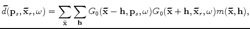 is an image point within the selected target zone;
 and
and
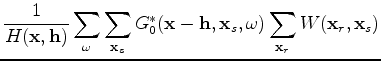
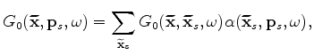
The synthesized areal data can be imaged by using conventional migration of areal-source data as follows:
 's are obtained using velocity model
 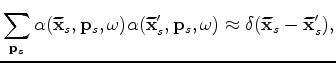 is the Dirac delta function. For plane-wave-phase encoding,
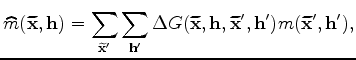
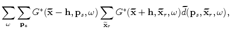
Substituting equations 4 and 3 into equation 5 yields
| (7) |
Throughout this paper, we perform numerical examples using
Green’s functions computed by means of one-way wavefield extrapolation
(Biondi, 2002; Stoffa et al., 1990; Claerbout, 1985; Ristow and Rühl, 1994).
Although not tested here, Green’s functions
obtained using other methods, such as by solving the two-way wave
equation, can also be used under this framework.
Since the one-way wavefield extrapolator has limited accuracy for large-angle propagation,
we only compute horizontal half subsurface offset, i.e.,
![]() .
.
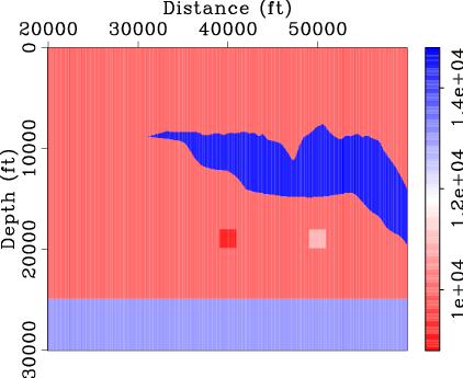
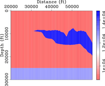
Figure 1(a) shows a modified Sigsbee2A velocity model, which contains two square anomalies below the salt:
one ![]() lower and the other
lower and the other ![]() higher than the sediment velocity.
We model
higher than the sediment velocity.
We model ![]() shots using the two-way wave-equation with a time-domain finite-difference scheme.
The data is recorded with a marine acquisition geometry, the maximum offset for each shot is about
shots using the two-way wave-equation with a time-domain finite-difference scheme.
The data is recorded with a marine acquisition geometry, the maximum offset for each shot is about ![]() ft.
We refer this two-way data set as ``original data'' hereafter. The migrated prestack image and gathers using the original data and a
starting velocity model (Figure 1(b)) are shown
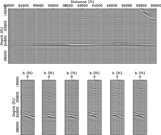
in Figure 2. The amplitude of the background image has been normalized by the diagonal of
the phase-encoded Hessian (equation 3) to partially compensate for uneven illumination (Tang, 2009).
Note the unfocused subsurface-offset-domain common-image gathers (SODCIGs) due to velocity errors.
Then we use the target image (Figure 2) and the Born modeling described above to generate
ft.
We refer this two-way data set as ``original data'' hereafter. The migrated prestack image and gathers using the original data and a
starting velocity model (Figure 1(b)) are shown
in Figure 2. The amplitude of the background image has been normalized by the diagonal of
the phase-encoded Hessian (equation 3) to partially compensate for uneven illumination (Tang, 2009).
Note the unfocused subsurface-offset-domain common-image gathers (SODCIGs) due to velocity errors.
Then we use the target image (Figure 2) and the Born modeling described above to generate
![]() plane-wave-source gathers from depth level
plane-wave-source gathers from depth level
![]() ft,
where the take-off angle is from
ft,
where the take-off angle is from
![]() to
to
![]() . The same starting velocity model that was used for migration
(Figure 1(b)) has been used for modeling,
and the new data set is collected just above the target region,
i.e.,
. The same starting velocity model that was used for migration
(Figure 1(b)) has been used for modeling,
and the new data set is collected just above the target region,
i.e.,
![]() ft. We refer to the Born-modeled data as ``new data'' hereafter.
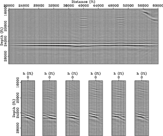
The plane-wave migration result of the new data set using the starting velocity model is shown in Figure 4.
Note the same kinematics shown in Figures 2 and 4.
This suggests that the velocity information has been successfully preserved using the new data set, which is substantially smaller compared
to the original one. Also note that Figure 4 is more blurry than Figure 2
due to the filtering effect of the resolution function
ft. We refer to the Born-modeled data as ``new data'' hereafter.
The plane-wave migration result of the new data set using the starting velocity model is shown in Figure 4.
Note the same kinematics shown in Figures 2 and 4.
This suggests that the velocity information has been successfully preserved using the new data set, which is substantially smaller compared
to the original one. Also note that Figure 4 is more blurry than Figure 2
due to the filtering effect of the resolution function ![]() (equation 8).
(equation 8).
|
|---|
|
bwi-sigsb2c-vmod,bwi-sigsb2c-bvel
Figure 1. (a) The modified Sigsbee2A velocity model and (b) the starting velocity model. [ER] |
|
|
|
|---|
|
bwi-sigsb2c-bimg-target-cpst
Figure 2. Initial image obtained using the original two-way finite-difference modeled data. The image has been normalized using the diagonal of the phase-encoded Hessian. Top: zero-subsurface offset image (stacked image), bottom: SODCIGs at surface location |
|
|
|
|---|
|
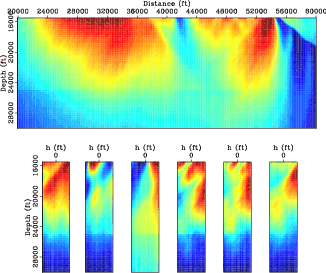
bwi-sigsb2c-bhes-target
Figure 3. The diagonal of the phase-encoded Hessian obtained using the background velocity model. View descriptions are the same as in Figure 2. [CR] |
|
|
|
|---|
|
bwi-sigsb2c-bimg-born-planes-target
Figure 4. The migrated image and gathers using the new data set. View descriptions are the same as in Figure 2. [CR] |
|
|
|
|
|
|
Target-oriented wavefield tomography using demigrated Born data |