Least-squares imaging and deconvolution using the hybrid norm conjugate-direction solver

Deconvolution of a common-offset field data

The second example is a common-offset section of field marine data. Figure 8 shows the input data.

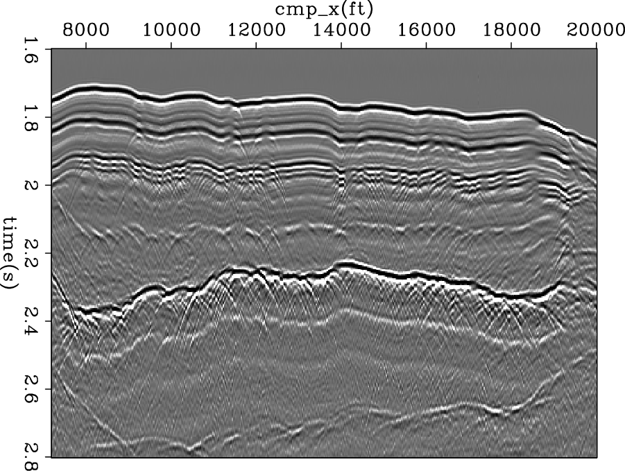
data-COF-decon
Figure 8. Input Common Offset data.

result-COF-decon
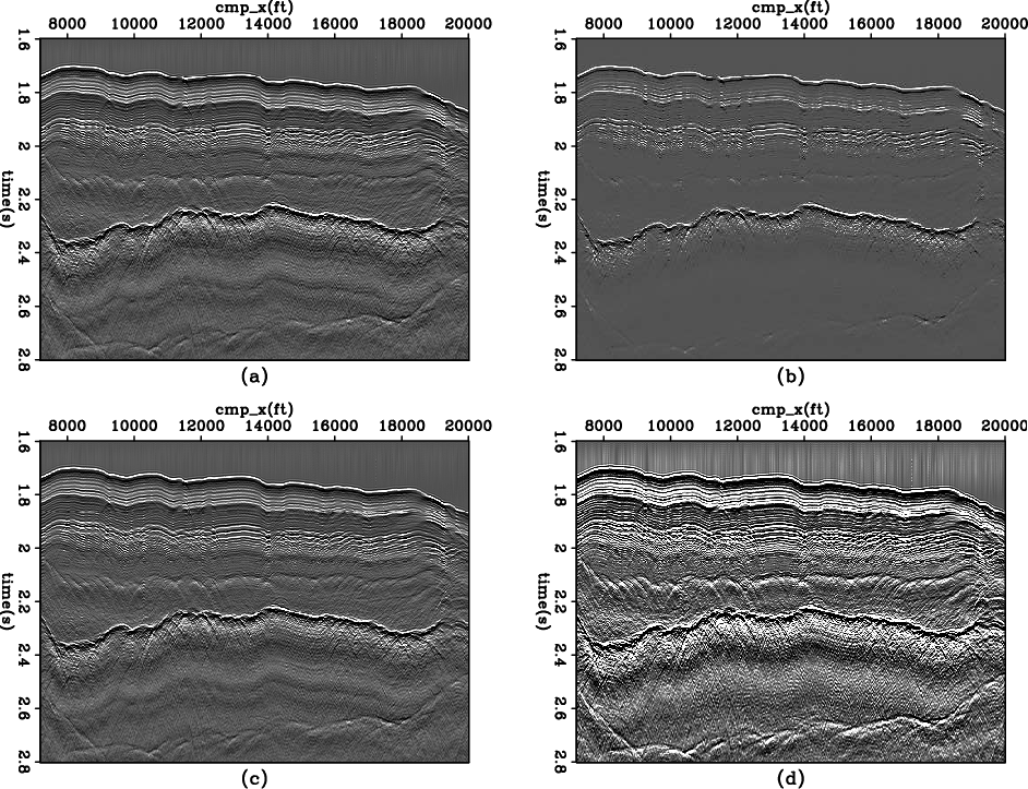
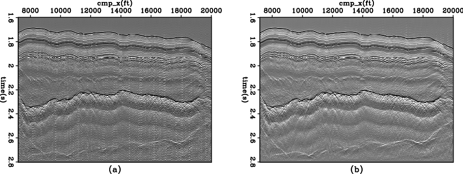
Figure 9. Top: L2 (a) and hybrid (b) deconvolution result for the Common Offset data; bottom: data fitting residuals of L2 (c) and hybrid (d) inversion.

Figure 9 shows the deconvolution result using L2 and L1 inversion. Although in this case the L1 inversion gives a cleaner model, the model is less desirable. Some areas of interest (like the salt-bottom) are suppressed by regularization due to lower amplitude than do the salt-top and sea-bed. In other words, the regularization is too strong. The bottom panel of Figure 9 showing the data fitting residual further confirms this point. From the amplitude information of this plot, roughtly 20% of the data was pushed into fitting error, the regularization distorts the data fitting too much rather than eliminating the model's null space.

single-trc-COF
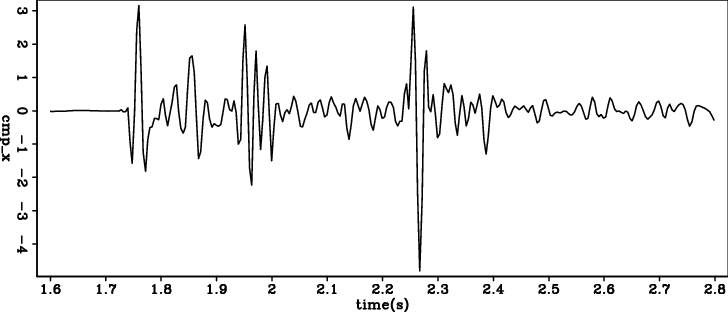
Figure 10. One single trace extracted at 12000m of the common offset section.

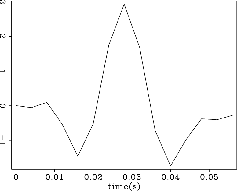
wav-man-COF Figure 11. The extracted source wavelet from seismic data.

res-mandecon-COF
Figure 12. (a): the L2 inversion result; (b) the hybrid inversion result.

Our predicament in this case is that if we set $\epsilon$ to a small value, then the hybrid result does not differ significantly from L2 result; on the other hand a large $\epsilon$ is not desirable either. Something in the data breaks our simple deconvolution model.

Figure 10 shows one trace extracted from the section. Thanks to the sparseness of the reflector, it is easy to identify the waveforms of several strong reflections. Take the very first sea bed reflection for instance, the wavelet is quite symmetric, more likely zero phase instead of minimum phase. From the lesson we have learned from the synthetic data, it is likely that the non minimum phase wavelet causes the failure of the method (4).

Fortunately, it is easy to identify the wavelets at several strong reflections, so we can roughly extract the wavelet from these locations and use this wavelet in the convolution model. The simplified inversion problem can be defined as follows:

$$\left\{ \begin{array}{ccc} \bold S \bold m & \approx & \bold d \bold \epsilon \bold m & \approx & \bold 0 \end{array} \right.$$ (5)

in which S is the convolution operator of the known wavelet s, m is the unknown model, and d is the seismic data.

Figure 11 shows the extracted source wavelet by averaging the wavelet at the sea-floor reflection among all traces. Figure 12 shows the result of L2 inversion and hybrid inversion. Compared with the orginal data, both deconvolution results improve the spatial resolution; and the hybrid result is less noisy than the L2 result.

Least-squares imaging and deconvolution using the hybrid norm conjugate-direction solver