|
 |
 |
 | Near-surface velocity estimation by weighted early-arrival waveform inversion |  |
![[pdf]](icons/pdf.png) |
Next: Examples
Up: Shen: Tomography
Previous: Introduction
The generalized waveform inversion objective function can be written as
 |
(1) |
where  is a function of
 , observed data and
 , forward modeled synthetic data from
  , the velocity model. Observed data can be in either the frequency domain or the time domain, depending on the actual form of
  . For example if we take
as the L2 norm of
. For example if we take
as the L2 norm of
 , we obtain the objective function of conventional waveform inversion (Tarantola, 1984; Pratt et al., 1998); if we take
as the L2 norm of natural logarithm of
, we obtain the objective function of conventional waveform inversion (Tarantola, 1984; Pratt et al., 1998); if we take
as the L2 norm of natural logarithm of
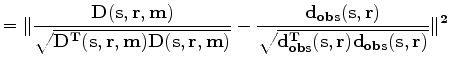
 , we obtain the so called logarithmic objective function of waveform inversion (Shin and Min, 2006). However, direct comparison in the phase domain will encounter the problem of phase wrapping. I modify the objective function of conventional waveform inversion by using the following expression for
:
, we obtain the so called logarithmic objective function of waveform inversion (Shin and Min, 2006). However, direct comparison in the phase domain will encounter the problem of phase wrapping. I modify the objective function of conventional waveform inversion by using the following expression for
:
where
is the model, which consists of near-surface velocity;
 are the data, which consist of band-passed early arrivals of the wavefield. Data are filtered based on traveltime difference before bandpassing to exclude events that come relatively late in the early arrivals.
  is the constant-density two-way acoustic wave-equation operator that generates synthetic early arrivals from source and near-surface velocity;
  and
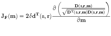
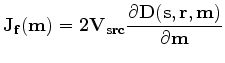
and  are source and receiver locations, respectively. In the new objective function, I weight both recorded data and forward-modeled data by their RMS energy trace by trace. This ensures that the recorded data and the forward-modeled data have relatively the same amplitudes, and waveform inversion in this case will focus more on phase comparison. To update the velocity, I use the nonlinear conjugate gradient method. The gradient of equation 2 with respect to
is as follows:
are source and receiver locations, respectively. In the new objective function, I weight both recorded data and forward-modeled data by their RMS energy trace by trace. This ensures that the recorded data and the forward-modeled data have relatively the same amplitudes, and waveform inversion in this case will focus more on phase comparison. To update the velocity, I use the nonlinear conjugate gradient method. The gradient of equation 2 with respect to
is as follows:
 |
|
|
(2) |
After some algebraic manipulations, equation 2 becomes:
 |
|
|
(3) |
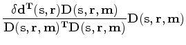
where
 is defined as
For gradient calculation, the only difference between conventional waveform inversion and weighted waveform inversion is how to calculate the virtual source. In conventional waveform inversion, the difference between observed data and modeled data is used as virtual source for reverse-time propagation. In weighted waveform inversion, a new virtual source defined in 5 is used for reverse-time propagation.
The step length calculation assumes local parabolic behavior of the objective function (Vigh and Starr, 2008). I first obtain two different perturbations of the velocity
 by scaling the gradient to about three percent of the minimum value in the current velocity; then I calculate the misfit function value, and determine the minimum of the parabola by using the two perturbation step length
 and
and
 and the existing velocity
 .
.
In the synthetic example shown next, I assume a known source wavelet in both examples. I carry out the waveform inversion using several frequency bands, starting from low frequency and gradually moving to higher frequency (Sirgue and Pratt, 2004). The inversion result of each frequency range is used as the starting model for inversion in the next frequency range. Using the low-frequency component of the data ensures good estimation of long-wavelength components of the velocity model, and subsequent higher-frequency inversion will retrieve finer velocity structures. As will be shown later, inversion results using this objective function are robust when we have attenuation or elastic waves in the recorded data.
|
|
|
|
| Near-surface velocity estimation by weighted early-arrival waveform inversion | |
|
Next: Examples
Up: Shen: Tomography
Previous: Introduction
2010-05-19