|
|
|
|
Low frequency passive seismic interferometry for land data |
|
geometry
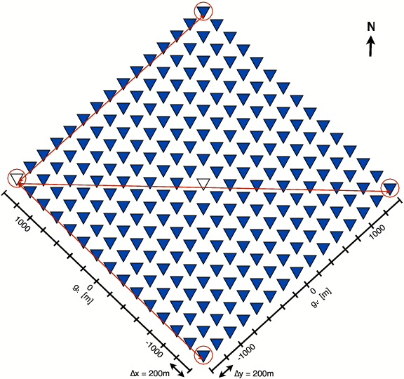
Figure 1. Geometry of the Aramco passive experiment; 225 stations (denoted by triangles) placed in a 15 by 15 grid. The geographic North is indicated by |
|
|---|---|
|
|
Stanford University received a nearly continuous raw data record spanning 48 hours divided over 3 days, starting on day 1 at 18:00 ending on day 3 at 18:00. Only vertical components were used, after removing the arithmetic mean over ![]() s time windows. The 48 hours of passive data were analyzed for their spectral characteristics. A frequency domain amplitude spectrogram averaged over the entire array is shown in Figure 2. Most energy was recorded between
s time windows. The 48 hours of passive data were analyzed for their spectral characteristics. A frequency domain amplitude spectrogram averaged over the entire array is shown in Figure 2. Most energy was recorded between ![]() Hz and
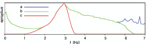
Hz and ![]() Hz and varies in a daily pattern with higher energy during the daylight hours and less energy at night. Figure 3 shows the frequency-domain amplitude spectrum, averaged for all recordings during the hour from 20:00 to 21:00 on day 1, drawn as curve (a). We identify a peak at very low frequencies, below 1 Hz.
Hz and varies in a daily pattern with higher energy during the daylight hours and less energy at night. Figure 3 shows the frequency-domain amplitude spectrum, averaged for all recordings during the hour from 20:00 to 21:00 on day 1, drawn as curve (a). We identify a peak at very low frequencies, below 1 Hz.

|
|---|
|
spectra1d-48-z
Figure 2. Frequency-domain amplitude spectrum averaged over the array as a function of time for 48 hours. White grid lines denote 6 hour blocks. a) Frequency-domain amplitude spectrum between 0 Hz and |
|
|
|
|---|
|
specbandpassed
Figure 3. Normalized frequency-domain amplitude spectrum, averaged over the array and data recorded between 20:00 and 21:00 on day 1. Curve (a) is the spectrum of the original data record, curve (c) is the spectrum after low-pass filtering for interferometry and curve (b) is the spectrum of the data after band-pass filtering for beam-forming. |
|
|
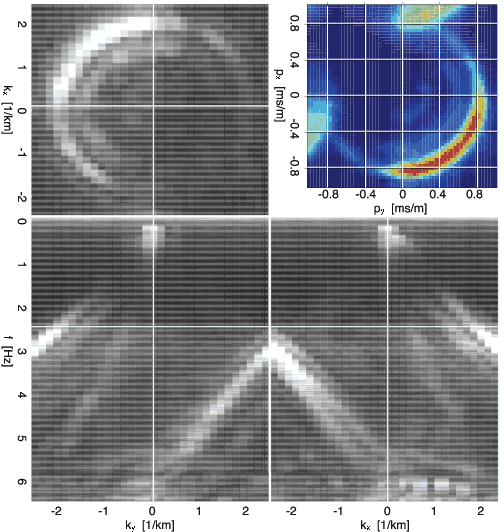
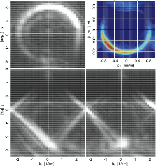
To help determine what kind of seismic energy composes the low-frequency spectrum, the frequency-wavenumber (![]() ) domain spectra were computed. A cross section through a cube of frequency-wavenumber spectra averaged over all recordings during the hour from 20:00 to 21:00 on day 1 is shown in Figure 4. The panel in the upper right corner of Figure 4 denotes a beam-forming experiment (see below). A cross section through a cube of frequency-wavenumber spectra averaged over all recordings between 11:00 and 12:00 on day 2 is shown in Figure 5. Both cross-sections only show frequencies below 6 Hz; above 6 Hz no wave modes could clearly be identified. Up to 6 Hz most of the energy resides in the (Rayleigh) surface wave modes. The fundamental mode becomes aliased above 3 Hz. Between 20:00 and 21:00 on day 1 most energy comes from the west, while from 11:00 to 12:00 on day 2 most energy comes from the north. (The directionality of the tails in the frequency-wavenumber spectra is controlled by the sign of the Fourier transformations.) Another common technique to characterize directionality in a wavefield is beam-forming. This was performed, after bandpass filtering between 1 Hz and 3.5 Hz, by computing linear
) domain spectra were computed. A cross section through a cube of frequency-wavenumber spectra averaged over all recordings during the hour from 20:00 to 21:00 on day 1 is shown in Figure 4. The panel in the upper right corner of Figure 4 denotes a beam-forming experiment (see below). A cross section through a cube of frequency-wavenumber spectra averaged over all recordings between 11:00 and 12:00 on day 2 is shown in Figure 5. Both cross-sections only show frequencies below 6 Hz; above 6 Hz no wave modes could clearly be identified. Up to 6 Hz most of the energy resides in the (Rayleigh) surface wave modes. The fundamental mode becomes aliased above 3 Hz. Between 20:00 and 21:00 on day 1 most energy comes from the west, while from 11:00 to 12:00 on day 2 most energy comes from the north. (The directionality of the tails in the frequency-wavenumber spectra is controlled by the sign of the Fourier transformations.) Another common technique to characterize directionality in a wavefield is beam-forming. This was performed, after bandpass filtering between 1 Hz and 3.5 Hz, by computing linear ![]() transformations over both directions. A beam is formed by averaging the amplitude in the
transformations over both directions. A beam is formed by averaging the amplitude in the ![]() domain over a certain
domain over a certain ![]() -window. (Note
-window. (Note ![]() denotes the interception times and
denotes the interception times and ![]() denotes the slownesses of the stacking lines of the
denotes the slownesses of the stacking lines of the ![]() transformation in
transformation in ![]() domain). The beams shown in the upper right corners of Figures 4 and 5 show that the fundamental mode travels with a slowness of slightly less than 1 ms/m (corresponding to a velocity of slightly greater than 1000 m/s). A higher mode visible in the frequency-wavenumber domain of Figure 4 can be observed (faintly) to travel with a slowness under 0.4 ms/m (corresponding with a velocity greater than 2500 m/s). Studying averaged frequency-wavenumber domains for other hours shows that the ambient seismic field at frequencies below 6 Hz is generally incident from the west and/or north.
domain). The beams shown in the upper right corners of Figures 4 and 5 show that the fundamental mode travels with a slowness of slightly less than 1 ms/m (corresponding to a velocity of slightly greater than 1000 m/s). A higher mode visible in the frequency-wavenumber domain of Figure 4 can be observed (faintly) to travel with a slowness under 0.4 ms/m (corresponding with a velocity greater than 2500 m/s). Studying averaged frequency-wavenumber domains for other hours shows that the ambient seismic field at frequencies below 6 Hz is generally incident from the west and/or north.
|
|---|
|
MDspectra1
Figure 4. Cross-sections through frequency-wavenumber spectra cube and averaged over the data recorded between 20:00 and 21:00 on day 1. The top right panel contains a beam-forming experiment for the frequency band of 1 Hz to 3.5 Hz. |
|
|
|
|---|
|
MDspectra2
Figure 5. Cross-sections through frequency-wavenumber spectra cube and averaged over the data recorded between 11:00 and 12:00 on day 2. The top right panel contains a beam-forming experiment for the frequency band of 1 Hz to 3.5 Hz. |
|
|
|
|
|
|
Low frequency passive seismic interferometry for land data |