|
|
|
|
Implicit finite difference in time-space domain with the helix transform |
where 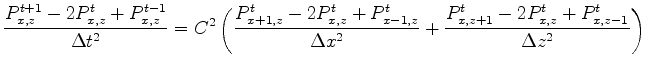 is the pressure wavefield,
 ![]() ,
, ![]() and
and ![]() are the time and space coordinate indices, and
are the time and space coordinate indices, and ![]() ,
, ![]() , and
, and ![]() are the temporal and spatial step sizes.
are the temporal and spatial step sizes.
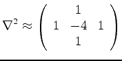
The 2D laplacian representing the spatial derivative's coefficients is:
In helical coordinates, the laplacian is represented as a sparse 1-D array:
Convolving this series with it's adjoint results in the following coefficients:
I used the SEPlib helicon module to convolve the coefficients in (4) with the data, coiling first in one direction, and then uncoiling in the other direction. The helicon module implements convolution by the linear operator:
where ![]() is the input data vector,
is the input data vector, 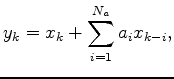 is a causal filter of length
 ![]() , and
, and ![]() is the output vector. The module also implements the adjoint:
is the output vector. The module also implements the adjoint:
where 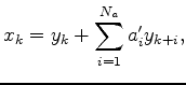 is the time reverse of filter
.
is the time reverse of filter
.
The application of the forward and reverse convolution replicates the act of using the standard finite differencing ``star'' to approximate the spatial derivative. The spatial derivative is then used to estimate the temporal derivative, and forward propagate in time the values of the acoustic wavefield.
With reference to Equation 1, the propagation kernel is:
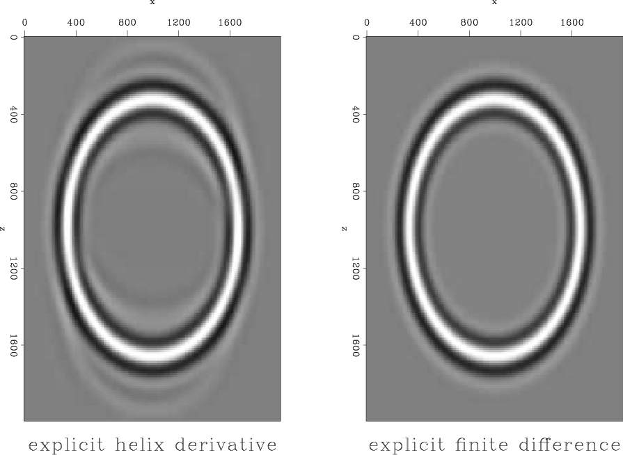
A comparison of propagation of a source in the center of a 2D acoustic wavefield with regular finite differencing and with the helix derivative is shown in Figure 2.
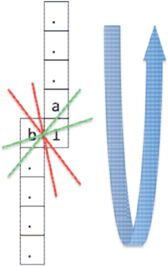
Although qualitatively the two results are similar, the wavefield created by the helix spatial derivative displays some form of dispersion both leading and trailing the main wavelet. Furthermore, the wavefront itself and the dispersion appear to be propagating anisotropically, with a slightly faster component along the positive diagonal. A possible explanation of this outcome is that the filter operator which convolves the data does not have a symmetric angular coverage. Refering to Figure 3, the better coverage of updip angles is apparent in comparison with downdip angles, as the filter is coiled around the data (in the direction of the arrow). If this is indeed the cause of dispersion, one way it can be mitigated is by using a cube finite differencing stencil (Haohuan et al. (2009)).
Another problem which is not apparent in Figure 2 is the wrap-around effect of the helix operator on the data being propagated. Since the helix wraps the filter convolution around one of the dimensions, it will invariably mix the information from one side of the wavefield with that from the other side. The longer and more accurate the filter will be, the more pronounced this effect will be as well. There is no immediate remedy for this inherent property of the helix, except for the standard model-padding solution. However, since the general intention is to use the helix for 2-way wavefield propagation in reverse time migration, one way the wrap around effect can be disregarded is by utilizing random boundaries in the wavefield, as shown in Clapp (2009).
|
|---|
|
exp-vs-hel-snap
Figure 2. comparison of 2nd order in time and space finite difference Vs. helix derivative after spectrally factorizing the coefficients of the 2nd order spatial derivative and convolving them with the data using helical boundaries. The propagation here is with constant velocity |
|
|
|
|---|
|
helical-aniso
Figure 3. Angular anisotropy of helical filter operator |
|
|
|
|
|
|
Implicit finite difference in time-space domain with the helix transform |