|
|
|
|
Joint least-squares inversion of up- and down-going signal for ocean bottom data sets |
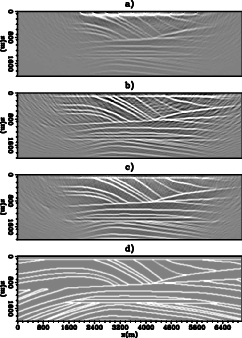
In this second example, we increase the spacing of the source and receiver array. There are 22 shots with a spacing of 300m spanning from 500-6800m. We use only 10 receivers that are 400 m apart and span from 2000-5600m. The model grid has a different reflectivity as shown in panel (d) of Figure 8. The rest of the parameters are the same as in the previous example.
Panel (a) and (b) of Figure 8 show the image from migration with the primary signal and with the mirror signal. In the up-image, we can see the strong near-surface amplitude, which is characteristic of the RTM. The down-image is coarse-grained due to the large shot and receiver spacings. Panel (c) of Figure 8 shows the corresponding joint inversion image (with 20 iterations). We can see a dramatic improvement from the joint inversion. This example demonstrates that when the recorded information is limited with respect to the complexity of the subsurface, joint inversion of up- and down-going signal can provide a better illuminated and more refined image.
|
|---|
|
sparseRTM
Figure 8. (a) The up-image, (b) the down-image, (c) the joint-image, and (d) the reflectivity model. |
|
|
|
|---|
|
sparseDeep
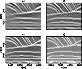
Figure 9. A close-up section of (a)The up-image (b) the down-image (c) the joint-image, and (d) the reflectivity model with coarse sampling. The sections are cut from x=2000-5000 m and y=500-1500 m. |
|
|
Figure 9 shows a close up section of Figure 8. It verifies the observation made in the previous example regarding the improvement of the joint-image.
|
|
|
|
Joint least-squares inversion of up- and down-going signal for ocean bottom data sets |