Marmousi model with dense sampling

Figure 6 (d) shows the reflectivity model used for this example. The model is 2 km deep and 7 km wide with a spacing of 10 m. The ocean floor is not included in this model and is assumed to be flat. However, it is possible to adapt the method to handle an ocean floor with topography. We use a water layer of 500m. All the images are generated in a target-oriented way. That means when we apply the RTM operator, we only cross-correlate regions below the sea-bottom. For simplicity, a constant velocity of 2500 m/s is used for this model.

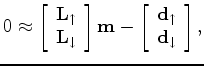
For the synthetic data, we use the $\mathbf L_{\uparrow}$ and $\mathbf L_{\downarrow}$ defined in the last section to forward model the lowest-order up-going (primary) and down-going (receiver ghost) data. In equation form, this is written as:

$\displaystyle \mathbf d_{\uparrow}^{mod}$	$\displaystyle =$	$\displaystyle \mathbf L_{\uparrow} \mathbf m$
$\displaystyle \mathbf d_{\downarrow}^{mod}$	$\displaystyle =$	$\displaystyle \mathbf L_{\downarrow} \mathbf m.$	(2)

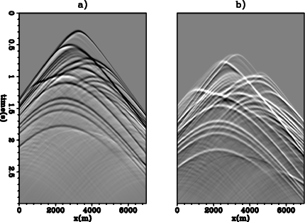
Shots run from 0 to 7000 m at the sea surface at an interval of 10 m. There are 700 shots in total. For the receiver geometry, we use a receiver spacing of 100 m with ocean bottom nodes located at every grid point from 2500 m to 4400 m. There are 20 nodes in total. Because reciprocity is used later, this geometry is equivalent to having 20 shots at the sea-bottom and 700 receivers at the sea-surface. Figure 5 shows the corresponding up-going and down-going common receiver gathers for a shot at x=3200 m.

To compare among conventional primary migration, mirror imaging, and joint inversion, we will first present the results of RTM on the conventional primary signal and on the mirror signal. The corresponding image will then be compared to the joint inversion result using both signals.