 |
 |
 |
 | Mechanics of stratified anisotropic poroelastic media |  |
![[pdf]](icons/pdf.png) |
Next: APPENDIX B: POROELASTIC FORMULAS
Up: Berryman: Stratified poroelastic rocks
Previous: SUMMARY AND CONCLUSIONS
The quasi-static elasticity equations are
often written in compliance form using the Voigt 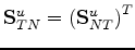 matrix
notation as:
matrix
notation as:
 |
(40) |
where  is the symmetric
compliance matrix.
The numbers 1,2,3 always indicate Cartesian axes (say,
is the symmetric
compliance matrix.
The numbers 1,2,3 always indicate Cartesian axes (say, 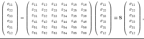 ,
, ,
, respectively).
The
-direction is usually chosen as the layering direction,
which could be oriented any direction in the earth.
But, in many geological and geophysical applications, the 3-axis (or
-axis)
is also taken to be the vertical direction, and I conform to this convention here.
The principal stresses are
respectively).
The
-direction is usually chosen as the layering direction,
which could be oriented any direction in the earth.
But, in many geological and geophysical applications, the 3-axis (or
-axis)
is also taken to be the vertical direction, and I conform to this convention here.
The principal stresses are
 ,
,
 ,
,
 ,
in the directions 1,2,3, respectively. Similarly, the principal strains
are
,
in the directions 1,2,3, respectively. Similarly, the principal strains
are  ,
,  ,
,  .
The stresses
.
The stresses
 ,
,
 ,
,
 are the torsional shear stresses,
associated with rotation-based strains around the 1, 2, or 3 axes, respectively.
The corresponding torsional strains are
are the torsional shear stresses,
associated with rotation-based strains around the 1, 2, or 3 axes, respectively.
The corresponding torsional strains are  ,
,  , and
, and
 , where the torsional motion is again a rotational straining motion around the
1, 2, or 3 axes.
The compliance matrix is symmetric, so
, where the torsional motion is again a rotational straining motion around the
1, 2, or 3 axes.
The compliance matrix is symmetric, so
 , and this fact
could have been used when displaying the matrix.
The axis pairs in the subscripts
, and this fact
could have been used when displaying the matrix.
The axis pairs in the subscripts  ,
,  ,
,  ,
,  ,
,  , and
, and  ,
are often labelled (again following the conventions of Voigt) as 1,2,3,4,5,6, respectively.
,
are often labelled (again following the conventions of Voigt) as 1,2,3,4,5,6, respectively.
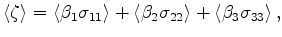
The important contribution made by Backus (1962) [also see Postma (1955)]
is the observation that, in a horizontally layered system, there are certain strains
 and stresses
 that are necessarily continuous
across boundaries between layers, while the others are not necessarily continuous.
I have been implicitly (and now explicitly by calling this fact out) assuming
that the interfaces between layers are in welded contact,
which means practically that the in-plane strains are always continuous:
so if axis 3 (or
) is the symmetry axis
(as is most often chosen for our layering problem), I have
,
that are necessarily continuous
across boundaries between layers, while the others are not necessarily continuous.
I have been implicitly (and now explicitly by calling this fact out) assuming
that the interfaces between layers are in welded contact,
which means practically that the in-plane strains are always continuous:
so if axis 3 (or
) is the symmetry axis
(as is most often chosen for our layering problem), I have
,
 , and
are all continuous.
Similarly, in welded contact, I must have continuity of the all the
stresses involving the 3 (or
) direction: so
,
, and
are all continuous.
Similarly, in welded contact, I must have continuity of the all the
stresses involving the 3 (or
) direction: so
,
 , and
, and
 must all be continuous.
Then, following Backus (1962) and/or Schoenberg and Muir (1989) but -- for present purposes considering instead the compliance (inverse of stiffness) matrix --
I have rearranged the statement of the problem so that:
 |
(41) |
Note that this equation, although similar to (40) is
nevertheless quite different because of the rearrangement of
the matrix elements and the reordering of the strains and stresses.
The expression in (41) is general for all elastic media.
In the main text I restrict the discussion to orthotropic media. Assuming then that
I am using the correct set of axes as the symmetry axes in the presentation,
all off-diagonal compliances having subscripts 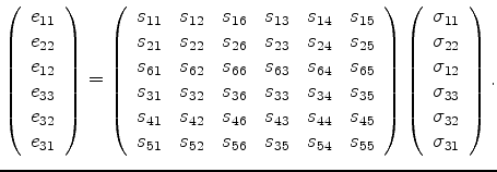 ,
,  , or
, or  in (40)
vanish identically. The diagonal shear compliances
in (40)
vanish identically. The diagonal shear compliances  , etc., generally do not vanish however.
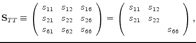
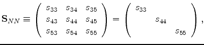
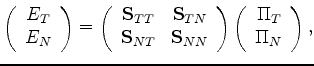
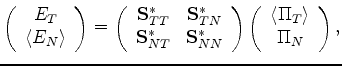
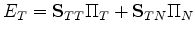
Expression of (41) can be made more compact by writing it as:
 |
(42) |
where
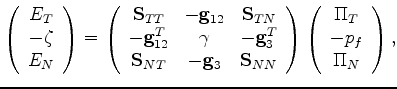 |
(43) |
 |
(44) |
and
 |
(45) |
with
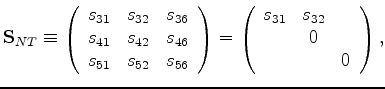 (with
(with  superscript indicating the matrix transpose).
Also I have
superscript indicating the matrix transpose).
Also I have
 |
(46) |
and
 |
(47) |
It is important to distinguish between ``slow'' and ``fast'' variables
in this analysis, since this distinction makes it clear when
and how averaging should be performed.
The ``slow'' variables, i.e., those that are continuous across the (here assumed horizontal)
boundaries and also essentially constant for the present quasi-static application, are
those contained in 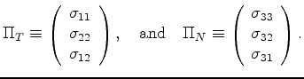 and
and  . So, after averaging
 along the layering direction, I have:
 |
(48) |
where
 , and
all the starred quantities are the nontrivial
average compliances I seek. They are defined in terms
of layer-average quantities where the symbol
indicates a simple volume average of all the layers. By this notation I mean
that a quantity
, and
all the starred quantities are the nontrivial
average compliances I seek. They are defined in terms
of layer-average quantities where the symbol
indicates a simple volume average of all the layers. By this notation I mean
that a quantity 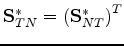 that takes on different values in different
layers has the layer average
that takes on different values in different
layers has the layer average
 .
The definition is general and applies to an arbitrary number of
different layers where the fraction of the total volume occupied
by layer
.
The definition is general and applies to an arbitrary number of
different layers where the fraction of the total volume occupied
by layer  is
is  , etc. Total fractional volume is
 .
.
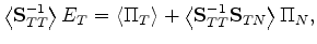
Of the three final results, the two easiest ones to compute are:
 |
(49) |
 |
(50) |
where
is the layer average of some quantity.
These results follow from this equation:
 |
(51) |
which also followed immediately from the formula
 |
(52) |
multiplying through first by the inverse of
 , and then performing the
layer average. [Note that
and
, and then performing the
layer average. [Note that
and
 are both
normally square and invertible matrices, whereas for most systems the
off-diagonal matrix
are both
normally square and invertible matrices, whereas for most systems the
off-diagonal matrix
 is not invertible. But, this fact does not cause problems
in the analysis, because I do not need to invert
in order to solve
the averaging problem at hand.]
These averages are meaningful because, when the matrix equations
presented are multiplied out, there never appear any cross products of two
quantities that are both unknown. [From this view point, Eq. (51)
is an equation for
is not invertible. But, this fact does not cause problems
in the analysis, because I do not need to invert
in order to solve
the averaging problem at hand.]
These averages are meaningful because, when the matrix equations
presented are multiplied out, there never appear any cross products of two
quantities that are both unknown. [From this view point, Eq. (51)
is an equation for
 , just as the unaveraged version of
(51) is an equation for
, just as the unaveraged version of
(51) is an equation for  in each layer.]
So simple layer-averaging suffices (thereby providing the main motivation and value
of this method).
Multiplying (51) through by
in each layer.]
So simple layer-averaging suffices (thereby providing the main motivation and value
of this method).
Multiplying (51) through by
 then gives
the results (49) and (50).
then gives
the results (49) and (50).
The remaining result is more tedious to compute, since it requires several intermediate steps
in its derivation. But the final result is given by the formula:
 |
(53) |
To provide some clues to the derivation, again consider:
 |
(54) |
which is just a rearrangement of (52). The point is that
is then given immediately in terms of the quantities
and
, which are both ``slow'' variables and therefore
essentially constant. An intermediate result that helps to explain
the form of this relation (53) is:
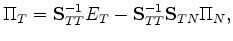 |
(55) |
Substituting for
from (54) into
 |
(56) |
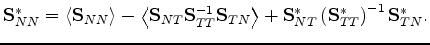
and then averaging, I find that
 |
(57) |
an expression that completely determines the remaining coefficients. After some more algebra,
the formula giving the final result is:
 |
(58) |
Equation (58) contains all the information needed to produce
the third and final result found in (53).
Another check on these formulas is to compare them directly to those found
by Schoenberg and Muir (1989). However, direct comparison is not so easy,
since their analysis focuses on the stiffness version of these equations.
My treatment makes use of the compliance version instead. Since the symmetries
of the two forms of the equations nevertheless are nearly identical, cross-checks
and comparisons will be left to the interested reader.
|
|
|
|
| Mechanics of stratified anisotropic poroelastic media | |
|
Next: APPENDIX B: POROELASTIC FORMULAS
Up: Berryman: Stratified poroelastic rocks
Previous: SUMMARY AND CONCLUSIONS
2010-05-19