 |
 |
 |
 | Mechanics of stratified anisotropic poroelastic media |  |
![[pdf]](icons/pdf.png) |
Next: SUMMARY AND CONCLUSIONS
Up: AVERAGING RESULTS FOR ALL
Previous: Drained scenario ( )
Now consider that the fluid pressure might vary across the stack of layers
(as should be expected to happen either because of hydrostatic overburden,
or due to fluid injection or extraction at certain chosen depths). Then I can treat this case as well,
assuming undrained circumstances, by averaging the fluid pressure itself via
 .
In this case, some knowledge of the fluid-pressure distribution along the stack of layers would be required,
as well as some information about whether the undrained condition applies at every interface, or just at some interfaces.
Variations might occur if a sealing layer were present to close off flow at the top, or bottom. Both ends might
be sealed for some range of porous layers forming a heterogeneous, layered anisotropic reservoir including cap rocks.
For this undrained case, the fluid pressure in each undrained layer is free to vary compared to all the others;
so there is no constancy of
.
In this case, some knowledge of the fluid-pressure distribution along the stack of layers would be required,
as well as some information about whether the undrained condition applies at every interface, or just at some interfaces.
Variations might occur if a sealing layer were present to close off flow at the top, or bottom. Both ends might
be sealed for some range of porous layers forming a heterogeneous, layered anisotropic reservoir including cap rocks.
For this undrained case, the fluid pressure in each undrained layer is free to vary compared to all the others;
so there is no constancy of  for this scenario. The averaging condition resulting from the formulation for such
a reservoir according to (29) is:
for this scenario. The averaging condition resulting from the formulation for such
a reservoir according to (29) is:
 |
(37) |
Proper choice of the range of depth for averaging will clearly depend on the details of each reservoir,
and the type of physical probe being used. For example, either quarter- or half-wavelength for seismic waves,
when used as the probe, would be typical choices of the averaging depth in this case.
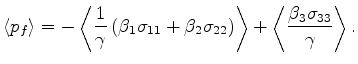
While the preceding part of the averaging for undrained boundary conditions was straightforward, I still
need to check what happens when averaging the remainder of the equations. I show the work in Appendix B
leading to the general undrained result (61), but just quote the final answer here -
being valid for each undrained layer in the overall system:
 |
(38) |
where
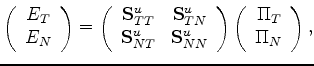 |
(39) |
while
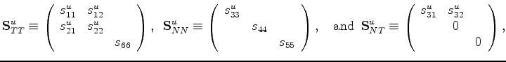 .
Once these definitions are used for the undrained matrices, the layer analysis for
the system follows exactly the same steps as in Appendix A. Note that I arrived
at these results in another (step-by-step) way in Appendix B in order to prove
that this is the right answer for the undrained problem. Fortunately, the intuitive
answer is also the same as the right answer.
.
Once these definitions are used for the undrained matrices, the layer analysis for
the system follows exactly the same steps as in Appendix A. Note that I arrived
at these results in another (step-by-step) way in Appendix B in order to prove
that this is the right answer for the undrained problem. Fortunately, the intuitive
answer is also the same as the right answer.
|
|
|
|
| Mechanics of stratified anisotropic poroelastic media | |
|
Next: SUMMARY AND CONCLUSIONS
Up: AVERAGING RESULTS FOR ALL
Previous: Drained scenario ( )
2010-05-19