Seismic reservoir monitoring with simultaneous sources

Conclusions

We have proposed an efficient scheme for acquiring and processing time-lapse seismic data sets. This method can reduce the overall data acquisition and processing cost for seismic reservoir monitoring. We have shown that even if the survey geometries and relative shot timing are not repeated, our joint inversion method gives high-quality time-lapse images. These acquisition and processing approaches provide a realistic framework for efficient seismic reservoir monitoring in many scenarios. It can make several conceptual seismic monitoring technologies (e.g. autonomous seismic acquisition, Arctic seismic reservoir monitoring) possible. In the near future, we will incorporate a scheme to compensate for geomechanical reservoir changes.

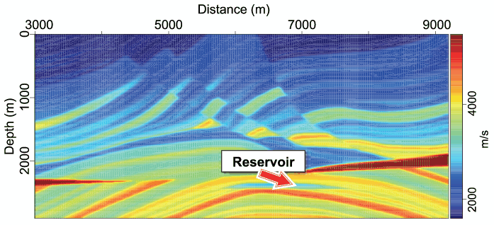
vel-0,dip-0,var-0
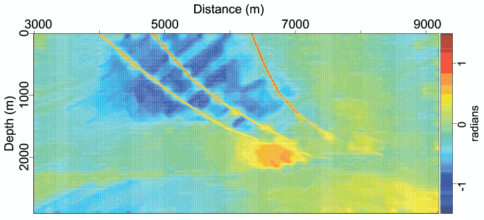
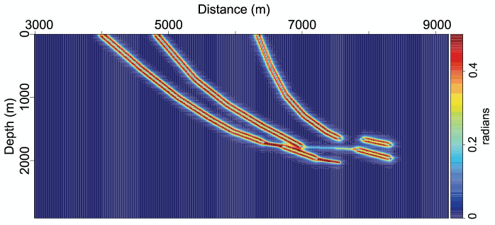
Figure 3. Baseline velocity model (a), dip-field computed from the migrated baseline image (b), and dip-variance estimated as a function of dip contrast (c). [CR].

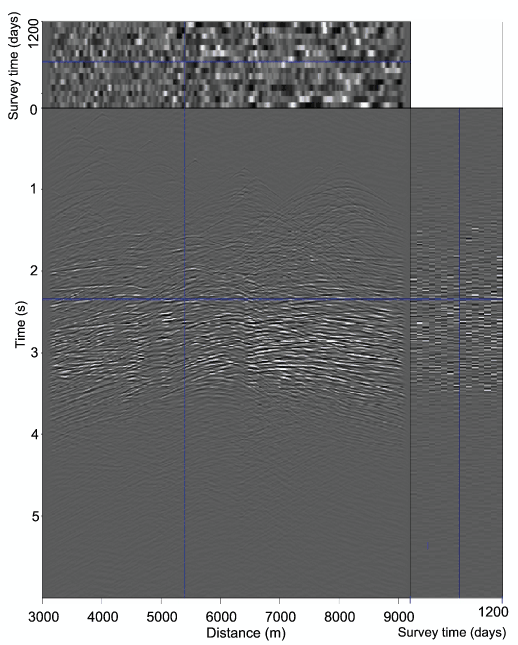
data-0
Figure 4. Synthetic data from multiple asynchronous sources. The third dimension denotes survey/recording time. [CR].

source-time
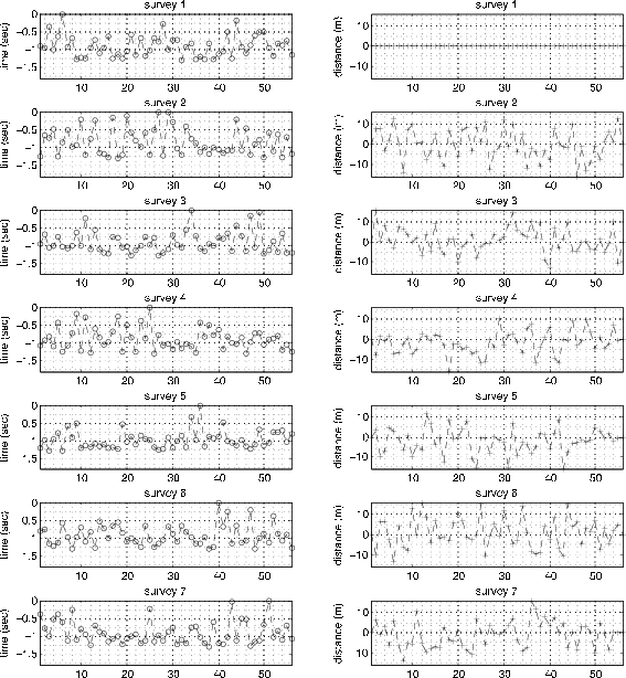
Figure 5. Plots of relative time-delays (left) and shot-displacements for seven out of the fifteen numerical models that were used to generate the data in Figure 4. In all plots, the horizontal axis indicates shot position. The relative shooting times are referenced to the earliest shot in each survey, whereas shot-displacements are referenced to the baseline shot positions. [NR].

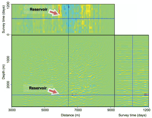
nomig,4d-nomig
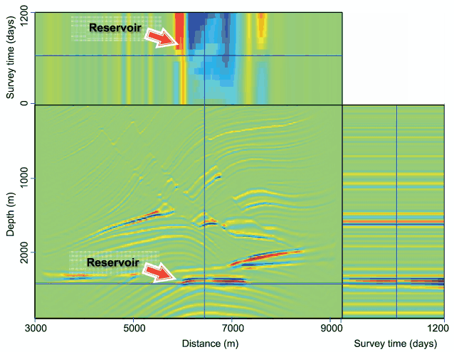
Figure 6. Images (a) and corresponding time-lapse estimates (b) obtained from migrating perfectly repeated conventional (single-source) data sets. In this (and in similar) Figures, the side panel (third axis) shows the seismic properties (a) and time-lapse changes (b) at a fixed spatial position, whereas the top panel shows the spatial-temporal distribution seismic properties. [CR].

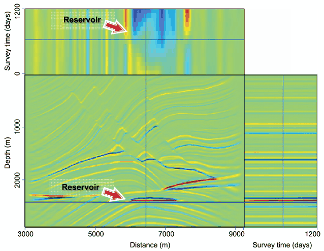
mig,4d-mig
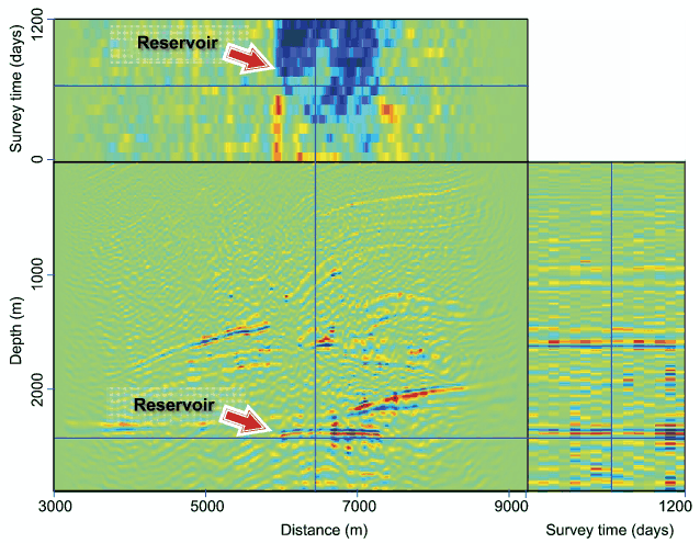
Figure 7. Images (a) and corresponding time-lapse estimates (b) obtained from migrating the data sets in Figure 4. In both Figures, note the numerous artifacts caused by geometry and shot-timing non-repeatability and cross-term artifacts. Without attenuating these artifacts, it would be difficult to accurately interpret the time-lapse information. [CR].

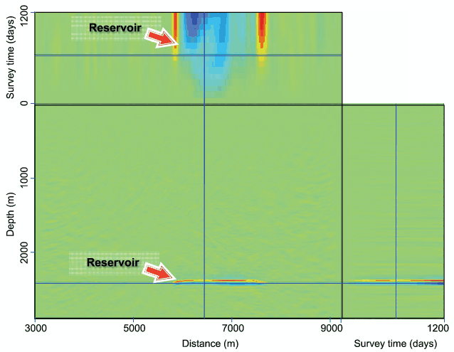
inv,4d-inv
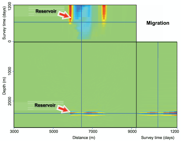
Figure 8. Images (a) and corresponding time-lapse estimates (b) obtained from inverting the simultaneous-source data sets in Figure 4. Note that the non-repeatability and cross-talk artifacts in the migrated images (Figure 7) have been attenuated by inversion. Also, note the better resolution of the inverted images compared to the migrated single-source data (Figure 6).

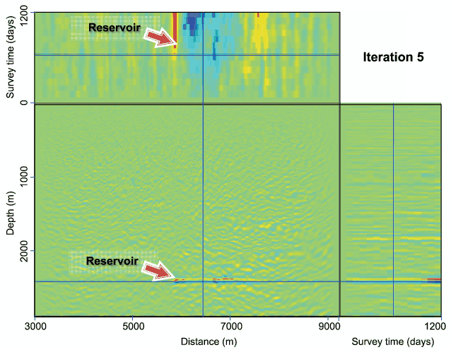
4d-inv-1,4d-inv-2
Figure 9. Time-lapse seismic images obtained after 2 and 5 conjugate gradient iterations (a) and (b) respectively. Note the gradual reduction in the artifacts compared to the time-lapse images from migration (Figure 7(b)). [CR].

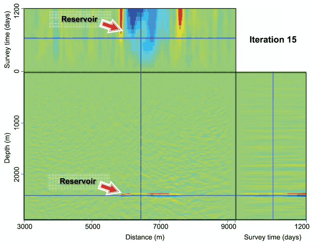
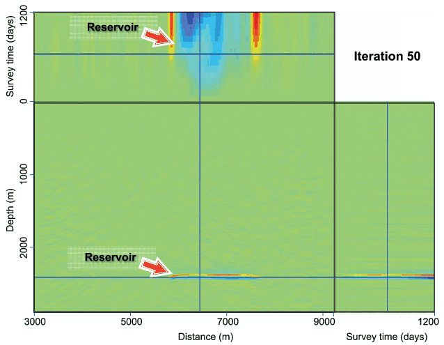
4d-inv-3,4d-inv-4
Figure 10. Time-lapse seismic images obtained after 15 and 50 conjugate gradient iterations (a) and (b) respectively. Note the reduction in the artifacts compared to the time-lapse images from migration (Figure 7(b)). [CR].

Seismic reservoir monitoring with simultaneous sources