Cyclic 1D matching of time-lapse seismic data sets: A case study of the Norne Field

Acknowledgements

Thanks to Statoil for the release of the Norne data. Thanks to the NTNU/IO CENTRE for their cooperation and coordination of the Norne Cases. Special thanks to Trine Alsos (Staoil), Mohsen Dadashpour (NTNU) and David Echeverria (Stanford Smart Fields) for their continued assistance throughout this study.

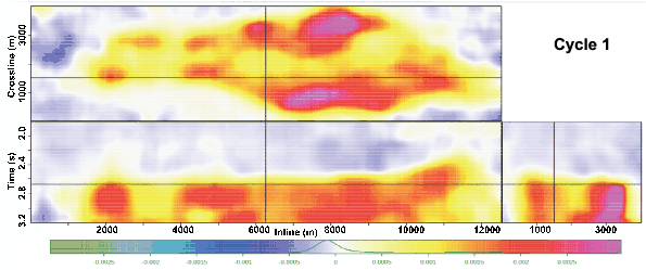
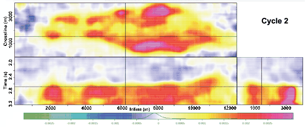
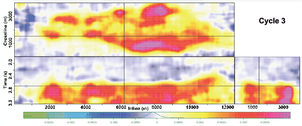
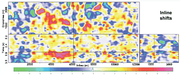
z-shift-1,z-shift-2,z-shift-3
Figure 1. Apparent vertical (time-) shifts estimates between the baseline and the 2006 data sets after one (top), tow (middle) and three (bottom) cycles. Note the improvement in resolution with the number of cycles. [CR].

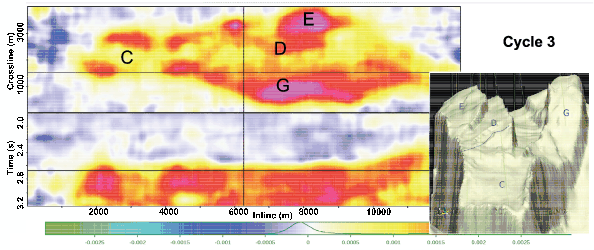
z-shift-3-TopNot
Figure 2. Time-shifts between the baseline and the 2006 data and the top of the reservoir. Note the similarity between the displacements correspond to known producing segments in the filed. [CR].

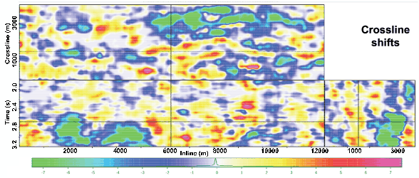
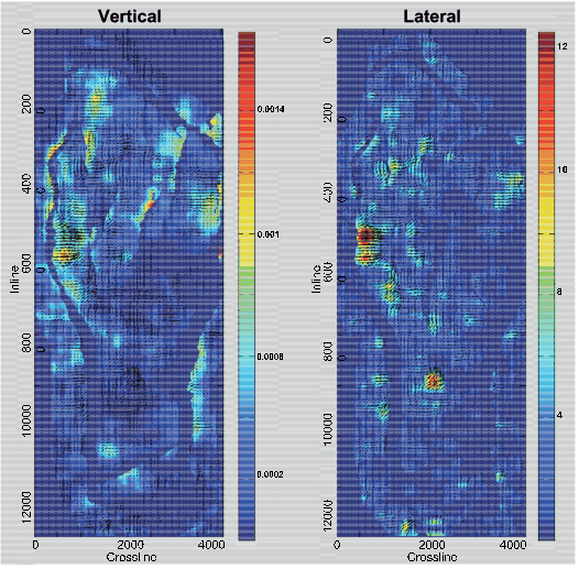
x-shift-3,y-shift-3
Figure 3. Apparent lateral displacements between the baseline and the 2006 data. [CR].

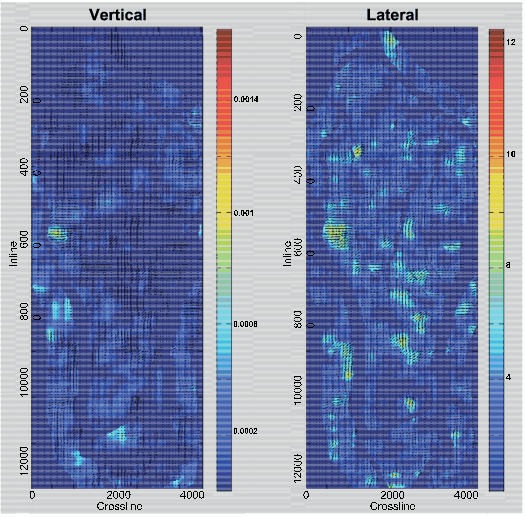
shift-compare1
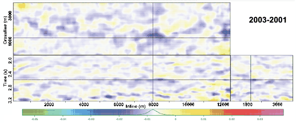
Figure 4. Absolute vertical and lateral displacements at the top of the reservoir between the baseline and the 2003 monitor. The arrows indicate the displacement direction. [CR].

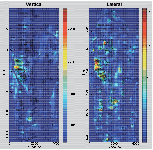
shift-compare2
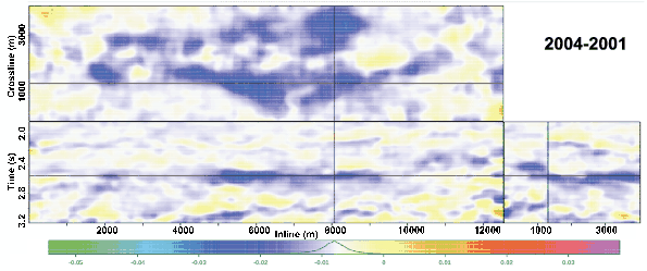
Figure 5. Absolute vertical and lateral displacements at the top of the reservoir between the baseline and the 2004 monitor. The arrows indicate the displacement direction. [CR].

shift-compare3
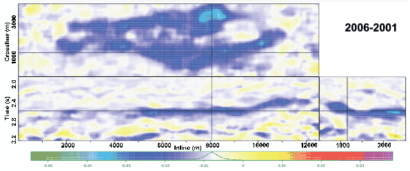
Figure 6. Absolute vertical and lateral displacements at the top of the reservoir between the baseline and the 2006 monitor. The arrows indicate the displacement direction. [CR].

dvv-shift-2003,dvv-shift-2004,dvv-shift-2006
Figure 7. Fractional velocity change between the baseline and the 2003 (a), 2004 (b) and 2006 (c) monitor data. Note that the velocity within the reservoir decreases with time. [CR].

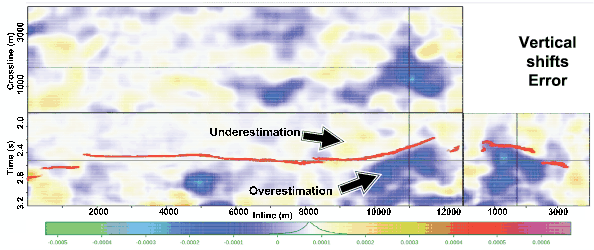
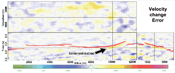
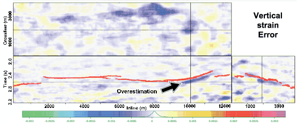
z-shift-3-error,dvv-shift-2006-error,ez-shift-2006-error
Figure 8. Time-shift (a), velocity change (b) and vertical strain (c) errors between the baseline and the 2006 data as a result of assuming on vertical displacements. In each case, the result obtained by considering only vertical displacements were subtracted from those obtained by considering all directions with the cyclic search method. The red line indicates the reservoir top. [CR].

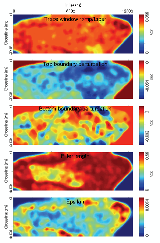
optimal-1
Figure 9. Optimal filter estimation parameters obtained by the evolutionary programming method. [CR].

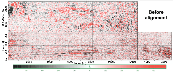
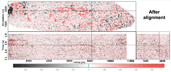
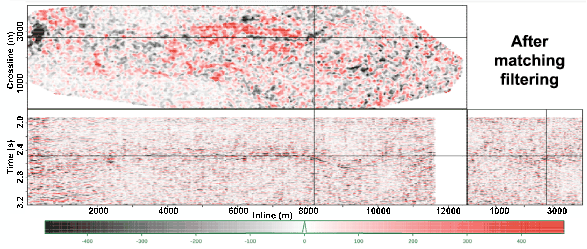
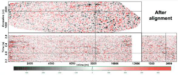
amp-shift-2006,amp-shift-2006-shifted,amp-shift-2006-matched
Figure 10. Time-lapse images after different processing steps. The top panel is a time-slice through the reservoir. Note the improvements in the quality of time-lapse amplitudes within the reservoir from top to bottom. [CR].

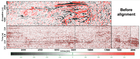
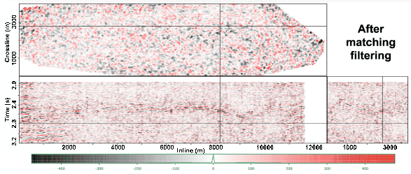
amp-shift-2006-b,amp-shift-2006-b-shifted,amp-shift-2006-b-matched
Figure 11. Time-lapse images after different processing steps. The top panel is a time-slice below the reservoir region where no time-lapse amplitude changes are expected. Note the improvement in the data quality from top to bottom. [CR].

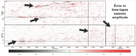
amp-shift-2006-b-error
Figure 12. Errors in time-lapse amplitude computed as a difference between the time-lapse image obtained by considering only vertical displacements and from considering all displacement components. [CR].

Cyclic 1D matching of time-lapse seismic data sets: A case study of the Norne Field