Geophysical applications of a novel and robust L1 solver

Simple Kirchhoff Inversion

Kirchhoff migration was widely used before the era of wave-equation migration for marine data, and is still the principle migration method for land data. It always involves summing over or spreading along certain travel-time surfaces in 3-D, which reduce to curves in 2-D. For the purpose of testing our solver, we define the forward operator to be the Kirchhoff modeling operator, whose adjoint is the traditional Kirchhoff migration operator.

We formulate the inversion problem as follows:

$${\bf H} {\bf m} \approx {\bf d}$$ (11)

$$\epsilon {\bf m} \approx {\bf0}$$ (12)

where $\bold H$ is the forward Kirchhoff modeling operator, $\bold m$ is the subsurface reflectivity model, and $\bold d$ is the seismic response recorded at the surface. The second equation is a damping term, where the hybrid-norm is applied to retrieve the sparse model.

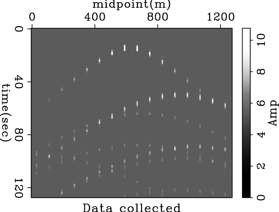
In field acquisition, data usually have denser sampling rates in the in-line direction than the cross-line direction. Therefore, the surface-recorded data are always aliased in the cross line direction. To illustrate the problem in the cross-line direction, figure 3 shows an example of highly aliased hyperbolas.The aliasing makes the inversion problem an underdetermined problem; therefore, the result of the inversion relies heavily on the regularization. With the model space sampling being $128 \times 128$ , the sampling of data space is only $128 \times 16$ . Also note that some of the hyperbolas are not symmetric; therefore the tops of the hyperbolas are shifted.

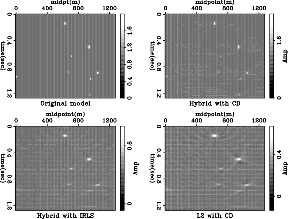
Same as the previous example, we experimented with different solvers: L2, IRLS and hybrid, to compare their results.

datasub
Figure 3. Highly aliased hyperbola. Input data for the Kirchhoff inversion.

show-mod-rand-8
Figure 4. Original model and inversion results by different methods. Top left: original model; Top right: Hybrid result with CD; Bottom left: Hybrid result with IRLS; Bottom right: L2 result with CD.

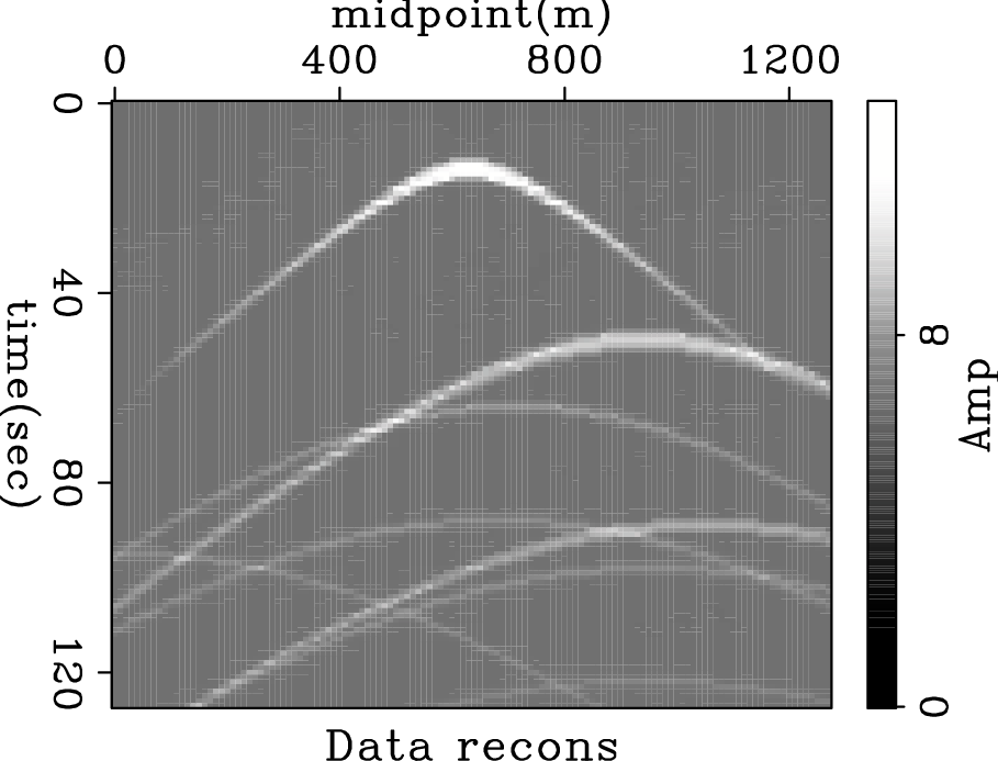
datahb Figure 5. Data reconstructed by the hybrid solver with CD. The CD hybrid solver accurately recovers the original data. Notice the hyperbola with its top at the left edge is well resolved.

Figure 4 shows the inversion results with different schemes. The results show that the hybrid norm is superior for retrieving the spiky result that resembles the original model the best. Although severely aliased, the inversion result recovers the exact position, the correct size and most of the amplitude. Notice that the CD hybrid solver recovers the very low amplitude spike at the left edge. This promising result suggests that by choosing the regularization properly, we can overcome the aliasing problem in the presence of a sparse model.

Figure 5 shows the reconstructed data from the CD hybrid solver. The original data are accurately recovered. Notice the hyperbola with its top at the left edge is well resolved.

Geophysical applications of a novel and robust L1 solver