Geophysical applications of a novel and robust L1 solver

Generalized conjugate direction method for the hybrid norm

The hybrid norm is defined as

$$h(r) = \sqrt{r^2+R^2}-R .$$ (1)

where $r$ is the residual, and $R$ is the corresponding threshold. In the limit, the hybrid norm (1) becomes:

$$h(r) = \left\{ \begin{array}{l l} \vert r\vert-R, \quad \mbox{if ... ...ert r\vert\ r^2/(2R), \quad \mbox{if } R \gg \vert r\vert. \end{array} \right.$$ (2)

It is obvious that when $R$ is small, the hybrid norm (1) reduces to L1 norm; when $R$ is big, it becomes the L2 norm. Therefore, threshold $R$ behaves as the turning point where the objective function changes smoothly from L2 to L1.

The Conjugate Direction method is commonly used for solving immense linear regressions in exploration geophysics. The idea of the CD method is to search the plane determined by the gradient and the previous step for the best step direction and length, instead of moving along the gradient direction. The best direction in that plane is the linear combination of the gradient and previous step vector that decreases the measure of the residual the most. Traditionally, the measure is chosen to be L2, for its simplicity; however, we generalize the CD method for any arbitrary convex measure 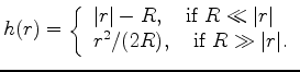$C$ . Readers can determine which measure to use to satisfy their own objectives.

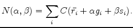
Now let us examine the generalization of the CD method in detail. At each iteration, we have the residual vector $\bar{r}$ , the gradient $g$ and the previous step $s$ . Therefore, the updated residual can be written as:

$$r_i = \bar{r_i} + \alpha g_i + \beta s_i.$$ (3)

where $\alpha$ and $\beta$ are scalars controlling the relative weights of these two directions. To determine these two scaling parameters, we need to minimize the measure of the residual:

$$N(\alpha,\beta) = \sum_i{C(\bar{r_i}+\alpha g_i + \beta s_i)}.$$ (4)

The system given by directly setting the partial derivatives of (4) to zero is transcendental, thus difficult to solve. Therefore, we use Taylor's expansion to approximate the original objective function. The polynomial estimation of (4) is given as follows:

$$N(\alpha,\beta) \approx \sum_i{ \bigg( C_i+(\alpha g_i + \beta s_i)C^{\prime}_i+(\alpha g_i + \beta s_i)^2 C^{\prime \prime}_i / 2 \bigg)}.$$ (5)

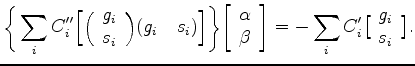
Now, taking the derivatives of the parabolic function in (5) with respect to $\alpha$ and $\beta$ and setting them to zero, we end up with a linear system of $\alpha$ and $\beta$ :

$$\bigg\{ \sum_i{C_i^{\prime \prime} \Big[ \Big( \begin{array}{l} g... ...] = -\sum_i{C_i^{\prime} \big[ \begin{array}{l} g_i \ s_i \end{array} \big] }.$$ (6)

where $(C_i,C_i',C_i'')$ refer to a Taylor expansion of $C(r)$ about $r_i$ .

Then we can obtain $\alpha,\beta$ by simply solving a set of 2 $\times$ 2 linear equations.

Notice that the $\alpha,  \beta$ we get here is minimizing the approximated function (5), not the original objective function. Therefore, it is necessary to solve for $\alpha,  \beta$ multiple times within each CD iteration. By doing this relatively cheap plane-search loop, we expect to save the number of iterations for the outer loop (Conjugate Direction), which is usually much more computational intensive (requiring application of both the forward and adjoint operator).

Geophysical applications of a novel and robust L1 solver