Fast 3D velocity updates using the pre-stack exploding reflector model

3D velocity update example

Migration velocity analysis by wavefield extrapolation using 3D PERM data was performed on a 3D real dataset from the North Sea with 3600 m maximum offset. This dataset was submitted to azimuth-moveout and imaged with CAM with an initial velocity sufficiently accurate up to the top of the chalk layer. From this reflector to deeper levels velocity is underestimated (Figure 5) as revealed by reflectors curving up in angle-domain common-image gathers at the bottom of Figure 6.

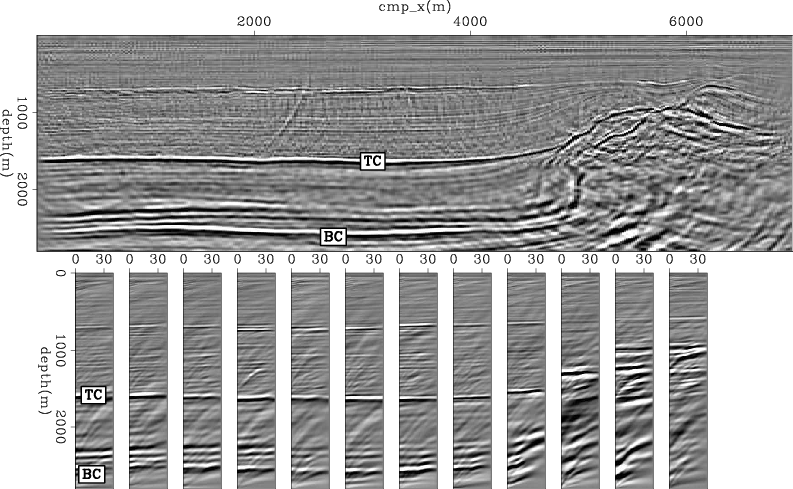
We compute velocity updates for the chalk layer in part of the 3D volume, which has 12 km in the in-line direction and 4 km in the cross-line direction. The velocity model definition for the entire 3D cube is ongoing work. We start by interpreting and windowing the base of chalk in the four-dimensional pre-stack image. The base of chalk is indicated by $\bf BC$ in Figure 6. The top of chalk, indicated by $\bf TC$ in Figure 6, is used as the upper limit for the velocity updates. The windowed reflector is then submitted to the rotation according to the apparent geological dip to correct for the image-point dispersal and it is used as the initial conditions to model 45 pairs of PERM source and receiver wavefields. Figure 7 shows the PERM receiver wavefield of one pair of wavefields. The wavefields are initiated by SODCIGs 1350 m apart. Since the offset range computed in the velocity optimization is 600 m, no crosstalk is generated. The wavefields are collected at 600 m depth, which is close to the top of the target-zone. Therefore, during the migration velocity analysis the wavefields are propagated between this depth level and the deeper level, which is 2800 m.

To optimize the velocity, we use a nonlinear conjugate gradient algorithm. The objective function we minimize is computed via differential-semblance optimization (DSO) (Symes and Carazzone, 1991; Shen and Symes, 2008), which corresponds to weighting the pre-stack image computed using the current velocity with the absolute value of the subsurface offset. The updated velocity is constrained to be within bounds 50$\%$ -lower and 50$\%$ -higher the initial velocity. Because of unbalanced amplitudes in the original data, it is necessary to smooth the gradient. We apply a B-spline smoothing, with node $xy$ -spacing of 1000 m. The optimization stopped after 5 iterations.

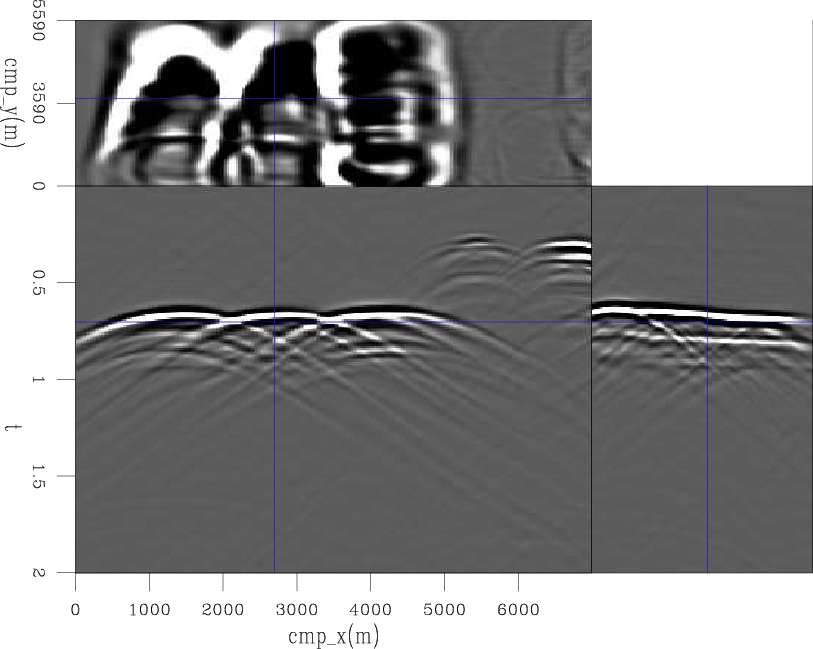
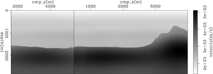
The optimized velocity model is shown in Figure 8 for the in-line at 3760 m and cross-line at 3500 m. Notice that, as expected, the optimized velocity is higher than the initial velocity. CAM using the optimized velocity confirms the correctness of the velocity update, by showing more focused reflectors and flatter ADCIGs than that obtained with the initial velocity (Figure 9). Compare with Figure 6. Some residual moveout is still present as can be seen in the rightmost ADCIGs of Figure 9. Since, the velocity of a salt body that occurs close to this region was not edited by a salt flooding procedure, we expect additional improvements in the image migrated with the final velocity model.

nsea03
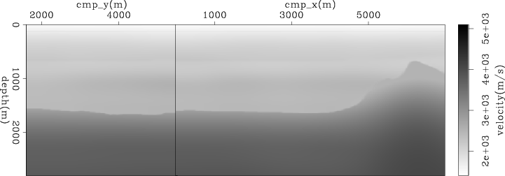
Figure 5. Initial velocity model. Left: cross-line at 3500 m. Right: in-line at 3760 m.

nsea01
Figure 6. Angle-gathers after CAM with the initial velocity. Top: zero-angle section. Bottom: ACDCIGs from $0^{\circ }$ to $40^{\circ }$ selected roughly at the same x position in the section above.

nsea00
Figure 7. PERM receiver wavefield of one areal shot.

nsea04
Figure 8. Optimized velocity model. Left: cross-line at 3500 m. Right: in-line at 3760 m.

nsea02
Figure 9. Angle-gathers after CAM with the optimized velocity. Top: zero-angle section. Bottom: ACDCIGs from $0^{\circ }$ to $40^{\circ }$ selected roughly at the same x position in the section above.

Fast 3D velocity updates using the pre-stack exploding reflector model