|
|
|
|
Wave-equation tomography by beam focusing |
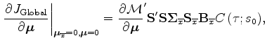
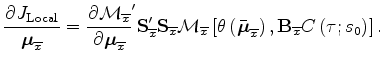
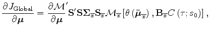
The computation of the derivatives of 3 with respect to each vector of local-moveout parameters is easily evaluated using the following expression:
 has the dimensions
![$ \stackrel{.}{C}\left({\tau};{s}_{0}\right)
=
C\left({\tau}\right)\left[
{\wide...
...}} }\left({t};{s}_{0}\right)
,
{\stackrel{.}{{P}}}_{D}\left({t}\right)
\right]
$](img64.png) ,
with
,
with
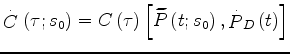 being the time derivative of the recorded-data traces.
For the choice of moveout parameters expressed in equation 6
we have
being the time derivative of the recorded-data traces.
For the choice of moveout parameters expressed in equation 6
we have
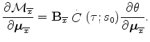
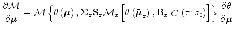
Similarly,
the evaluation of the derivatives of 7
with respect to each shift parameter
![]() is easily carried out by the following:
is easily carried out by the following:
 is given by
 .
.
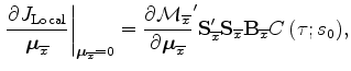
On a practical note, the preceding expressions look more daunting
than they are in practice.
They greatly simplify in the important case
when the gradient is evaluated for
![]() and
and
![]() .
This simplifying condition is actually always fulfilled
unless the optimization algorithm includes inner iterations
for fitting the moveout parameters using a linearized approach.
Under these conditions,
equations 12 and 13
become, respectively,
.
This simplifying condition is actually always fulfilled
unless the optimization algorithm includes inner iterations
for fitting the moveout parameters using a linearized approach.
Under these conditions,
equations 12 and 13
become, respectively,
|
|
|
|
Wave-equation tomography by beam focusing |