|
|
|
|
Wave-equation tomography by beam focusing |
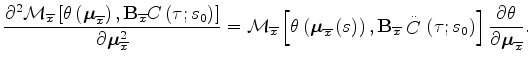
In this appendix I present the analytical development needed to derive equations 22-23 from equations 20-21.
Equation 20 can be rewritten as
 |
|||
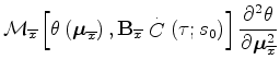
where,
![$\displaystyle \frac
{\partial^2\mathcal M_{\overline{x}}\left[
{\theta}\left({\...
...ft({\tau};{s}_{0}\right)
\right]}
{\partial {\boldsymbol \mu}_{\overline{x}}^2}$](img105.png) |
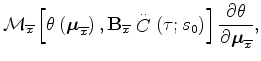
![$\displaystyle \mathcal M_{\overline{x}}\left[
{\theta}\left({\boldsymbol \mu}_{...
...
\right]\frac{\partial^2 {\theta}}{\partial {\boldsymbol \mu}_{\overline{x}}^2}$](img106.png) |
||
 |
![$ \stackrel{..}{C}\left({\tau}\right)
=
C\left({\tau}\right)\left[
{\widetilde{{P}} }\left({t}\right)
,
{\stackrel{..}{{P}}}_{D}\left({t}\right)
\right]
$](img86.png) .
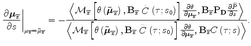
Given the moveout parametrization expressed in 6,
.
Given the moveout parametrization expressed in 6,
 and the previous
expression simplifies into the following:
and the previous
expression simplifies into the following:
 |
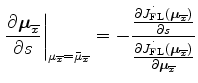
Similar derivation can be developed for the derivative of the global moveout parameters with respect to slowness. Equation 21 can be rewritten as:
 | |||
![$\displaystyle =
-\frac
{
\left\langle
\left.
\frac
{\partial
{
\mathcal M\left\...
...ht)
,{\bf B}_{\overline{x}}
C\left({\tau};{s}\right)
\right]
}
\right\rangle
},$](img113.png) |
|||
where,
![$\displaystyle {
\frac
{\partial^2
{
\mathcal M\left\{
{\theta}\left({\boldsymbo...
...ft({\tau};{s}_{0}\right)
\right]
\right\}
}}
{\partial {\boldsymbol \mu}^2}
=
}$](img114.png) | |||
![$\displaystyle \mathcal M\left\{
{\theta}\left({\boldsymbol \mu}\right)
,{\bolds...
...ight)
\right]\right\}\frac{\partial^2 {\theta}}{\partial {\boldsymbol \mu}^2}
+$](img115.png) |
|||
![$\displaystyle \mathcal M\left\{
{\theta}\left({\boldsymbol \mu}\right)
,{\bolds...
...{0}\right)
\right]\right\}\frac{\partial {\theta}}{\partial {\boldsymbol \mu}}.$](img116.png) |
|||
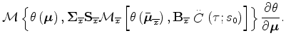 and the previous
expression simplifies into:
and the previous
expression simplifies into:
| |||
|
|||
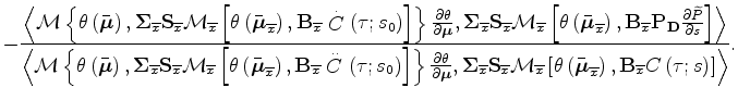
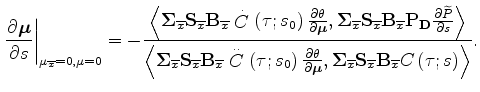
The general expression for the gradient of the global moveout parameters with respect to the slowness model is:
![$\displaystyle -\frac
{
\left\langle\mathcal M\left\{
{\theta}\left(\bar{{\bolds...
...ht)
,{\bf B}_{\overline{x}}
C\left({\tau};{s}\right)
\right]
}
\right\rangle
}.$](img119.png) |
|||
When
![]() and
and
![]() the general expression
further simplifies into:
the general expression
further simplifies into:
![]()
|
|
|
|
Wave-equation tomography by beam focusing |