|
|
|
|
Predicting rugged water-bottom multiples through wavefield extrapolation with rejection and injection |
Because the basic theory and extrapolation operator based on the Kirchhoff integral are widely known (Schneider, 1978; Margrave and Daley, 2001; Berkhout, 1981), I derive only the formulae corresponding to upward and downward wavefield extrapolation of both the up-going and down-going waves.
In general, the wavefield extrapolation from depth ![]() to
to
![]() can be written as follows:
can be written as follows:
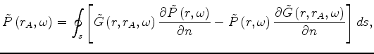
On the other hand, the Kirchhoff integral in the space-frequency domain is
 and
and
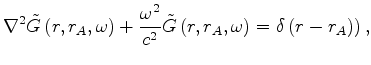 is wave propagation velocity. Obviously, it is not easy to relate equation 3 to the upward and downward wavefield extrapolation of both the up-going and down-going waves.
Suppose
is wave propagation velocity. Obviously, it is not easy to relate equation 3 to the upward and downward wavefield extrapolation of both the up-going and down-going waves.
Suppose
 and
and
 and
and Using the definitions of the down-going and up-going waves,
Thus the four types of wavefield extrapolations in terms of the Kirchhoff integral can be easily defined based on equation 11, as shown in figure 3.
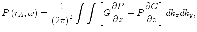
In practice, generally we transform the equation 11 from the (![]() ,
,![]() ,
,![]() ,
,![]() ) domain back into the(
) domain back into the(![]() ,
,![]() ,
,![]() ,
,![]() ) or (
) or (![]() ,
,![]() ,
,![]() ,
,![]() ) domain In this case, the down-going and up-going Green’s functions will change accordingly, as shown in figure 3. The terms
) domain In this case, the down-going and up-going Green’s functions will change accordingly, as shown in figure 3. The terms 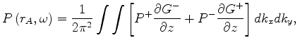 and
and ![]() are the causal and anticausal Green’s functions , or the “out-going ” and “in-going ” waves respectively.
are the causal and anticausal Green’s functions , or the “out-going ” and “in-going ” waves respectively.
After the above derivation, we have all types of wavefield extrapolations in terms of the Kirchhoff integral. In water-bottom multiple prediction, we use only types (a) and (c), that is, the downward wavefield extrapolation of the down-going wave and the upward wavefield extrapolation of the up-going wave.
|
|---|
|
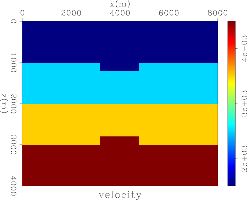
vel
Figure 4. The structure and interval velocity of the geological model. [NR] |
|
|
|
|---|
|
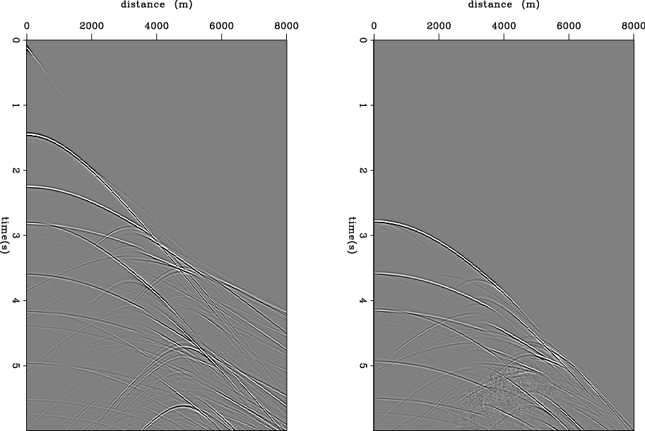
shotmult1
Figure 5. The shot gather at the leftmost location(left) and predicted multiples (right). [NR] |
|
|
|
|---|
|
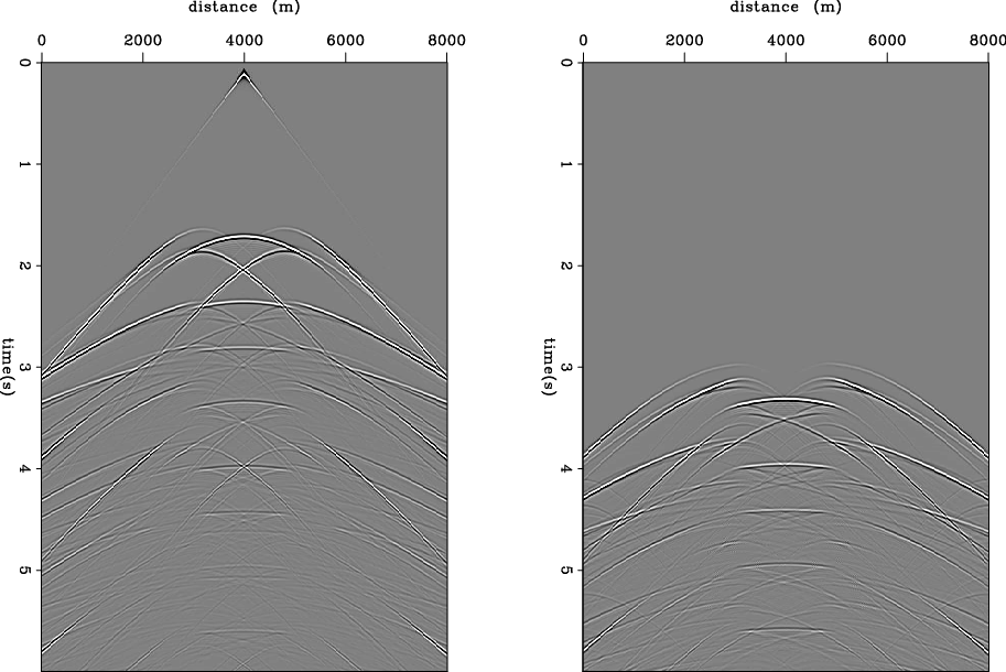
shotmult2
Figure 6. The shot gather at the central location (left) and predicted multiples (right). [NR] |
|
|
|
|
|
|
Predicting rugged water-bottom multiples through wavefield extrapolation with rejection and injection |
![$\displaystyle P\left(r_A,\omega\right) = \frac{1}{\left(2\pi\right)^2}\int\int\...
...tial{z}}} \ -P^-\frac{\partial{G^+}}{{\partial{z}}}\right)\right]dk_xdk_y, \ $](img45.png)
![$\displaystyle P\left(r_A,\omega\right) = \frac{1}{2\pi^2}\int\int\left[P^+\frac...
...{{\partial{z}}} \ +P^-\frac{\partial{G^+}}{{\partial{z}}} \right]dk_xdk_y, \ $](img46.png)