|
|
|
|
Applications of the generalized norm solver |
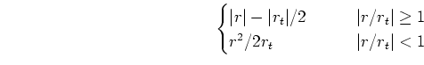
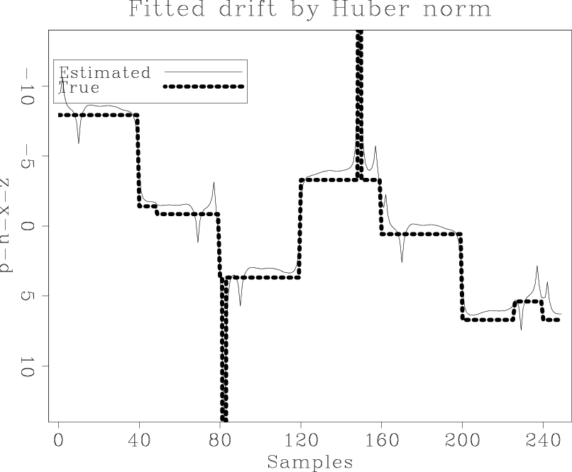
From observating the fitted drift between figure 6 (b) and 6 (d) , the Huber solver is not doing significantly better than the least-squares solver. One possible explanation is that the underlying Taylor series assumption failed while trying to solve for the stepping coeficient  and
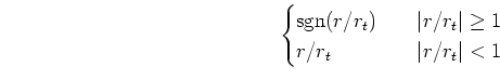
and ![]() . Recall that the formulas for the Huber norm are
. Recall that the formulas for the Huber norm are
| (5) | |||
 |
(6) | ||
 |
(7) |
Notice that the second derivative vanishes if the residual falls to the threshold value 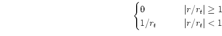 . This could lead to failure of the Huber solver, because the second derivatives are used in the denonimator when solving for the step size and
 ![]() in the conjugate-direction scheme (Claerbout (2009)).
in the conjugate-direction scheme (Claerbout (2009)).
We are delighted to see that hybrid solver gives a resonable result for the full Galilee problem as shown in figure 5(c), we can hardly describe the model solution as ``blocky." This might be because we have used a small threshold value for the model-fitting goal. For example, a threshold value of 0.30 percentile means we would like to see blocks about 3 to 4 points long. A higher threshold value for the model-fitting goal (equation 4) can increase blockiness; however our present solver has restricted us to use the same threshold value for both the model-fitting and the data-fitting goals (equation 3). One possible improvement for the future is to separate the thresholds for these goals.


|
|---|
|
norm-dpt0,norm-drf0,norm-dpt1,norm-drf1,norm-dpt2,norm-drf2
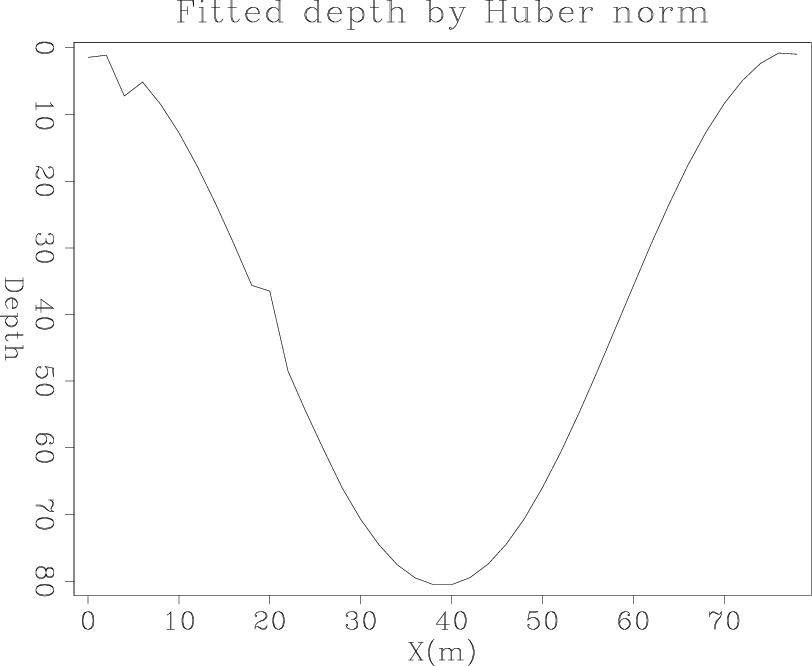
Figure 6. Fitting depth and drift for measurements with both drift and spiky noise with the generalized norm solver (regularized system) using the L2 norm (a,b); the Huber norm with |
|
|
|
|
|
|
Applications of the generalized norm solver |