|
|
|
|
Dix inversion constrained by L1-norm optimization |
Choosing proper parameters for hybrid  method and IRLS is still
quite empirical, even when we understand their physical
meanings. Instead, conjugate direction methods do not need setting
parameters. Thus, we develop a similar conjugate direction method in
method and IRLS is still
quite empirical, even when we understand their physical
meanings. Instead, conjugate direction methods do not need setting
parameters. Thus, we develop a similar conjugate direction method in ![]() sense. The pseudo code of this method is given in Table
1.
sense. The pseudo code of this method is given in Table
1.
The structure of the conjugate-direction ![]() method is similar to the
method is similar to the ![]() conjugate-direction solver given by Claerbout (2008). The main
difference arises in the part of plane search.
conjugate-direction solver given by Claerbout (2008). The main
difference arises in the part of plane search.
Given the gradient
![]() , previous step
, previous step
![]() , and
the current residual
, and
the current residual
![]() , we construct
the
, we construct
the ![]() matrix
matrix
![]() and the column
vector
and the column
vector
![]() . We seek to find
. We seek to find
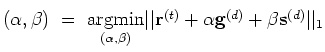
![]() that
minimizes
that
minimizes
![]() in the
L1-norm sense. This bivariate regression embedded in the plane search
is solved in an iterate manner.
in the
L1-norm sense. This bivariate regression embedded in the plane search
is solved in an iterate manner.
At the ultimate solution of the bivariate regression there will be two basis equations that are exactly satisfied. The first one is found by steepest descent. After the first iteration, we do plane searches using the weighted median solver to choose the best equation to be exactly satisfied. ``Best equation'' is the one that decreases the residual the most, while satisfying the equation chosen by the previous iteration exactly as well.
To do this, suppose the previous equation is
![]() . We seek a
. We seek a
![]() that still satisfies the equation
that still satisfies the equation ![]() . This requirement
gives a solution to
. This requirement
gives a solution to
![]() as
as
![]() , where
, where ![]() is a
scalar. Then the plane search becomes
is a
scalar. Then the plane search becomes
![]() , which is a weighted
median problem. Thus, using the weighted median solver, we can solve for
, which is a weighted
median problem. Thus, using the weighted median solver, we can solve for ![]() and
get a new equation, e.g., equation
and
get a new equation, e.g., equation ![]() . Then we can update
. Then we can update
![]() and
and
![]() accordingly, drop the old equation
accordingly, drop the old equation ![]() , and keep the new equation
, and keep the new equation
![]() . We iterate on this process until the inner loop keeps tracking the same
equation. The final results of the inner loop are
passed out to update the model, residual and the gradient.
. We iterate on this process until the inner loop keeps tracking the same
equation. The final results of the inner loop are
passed out to update the model, residual and the gradient.
The value of expending more effort to find the best step direction will be supported by the real geophysical applications, because the most computationally expensive part of these iterative methods is applying the forward and adjoint operators (steps starred in Table 1). By doing the sophisticate plane search, we hope to decrease the number of outer-loop iterations required for convergence.
However, conjugate direction L1 regression theory is not perfect for a
practical problem. The problem of a flat bottom in ![]() minimization
will cause trouble in geophysical practice. Sometimes
even where the bottom is not exactly as flat as the median of an even
number of points, the slope of the gradient can be so small that we
can never reach convergence in a finite number of iterations.
minimization
will cause trouble in geophysical practice. Sometimes
even where the bottom is not exactly as flat as the median of an even
number of points, the slope of the gradient can be so small that we
can never reach convergence in a finite number of iterations.
|
|
|
|
Dix inversion constrained by L1-norm optimization |