Measuring velocity from zero-offset data by image focusing analysis

New York harbor data example

I tested the method for extracting velocity information from zero-offset data on a shallow seismic data set acquired in New York harbor using a 512i sub-bottom profiler with a 1-10 kHz pulse (Schock et al., 1994,1989). Compared with conventional exploration data, these data contain much higher frequencies (useful signal is up to about 2,000 Hz) and have been acquired with correspondingly dense, though quite irregular, spatial sampling. For the sake of simplicity, I assumed that the acquisition grid was regular with spatial sampling of 0.225 meters; that is, the average of the actual sampling for the subset I analyzed. The actual standard deviation of the spatial sampling is about 0.018 meters; that is, about 8%.

Figure 5 shows the subset of the data that I worked with. The water bottom primary reflection is recorded at about 18 milliseconds; strong multiple reflections are visible below the primaries. From nearby well-boring, the layered body in the middle is thought to be composed by Holocene sediments, mostly sands, with velocity of approximately 2.150 km/s. The sediments are surrounded by serpentinite that has much higher seismic velocity. The serpentinite velocity ranges from 2.500 km/s where the rock is fractured (on the left of the sediments) to 4.300 km/s, where the rock is intact (below the sediments).

I first migrated the data assuming a constant velocity equal to the velocity of water; that is, 1.500 km/s. Figure 6 shows the depth-migrated section. The diffraction-like events visible in the data just after the water-bottom reflection are properly focused in the migrated section. The deeper events show some sign of undermigration, but it is difficult to judge with certainty.

I performed the focusing analysis described earlier in the paper on a small analysis window; this window was centered on the events at flattish sediment-serpentinite interface at the bottom of the sediment layers. The depth of the analysis window ranged from 21 to 25 meters, for the first iteration. I adjusted the depth for the following iterations to ensure that the analysis windows consistently included the same reflectors across iterations. To avoid artifacts caused by the noisy traces clearly visible in the data around the midpoint location of 126 meters, I further limited the analysis window horizontally, to span only the midpoint interval between 87 to 126 meters.

Data3-overn
Figure 5. Zero-offset data recorded in New York harbor using a 512i sub-bottom profiler with a 1-10 kHz pulse. [CR]

Mig-water-overn
Figure 6. Depth-migrated section obtained assuming a constant velocity equal to the velocity of water; that is, 1.500 km/s. [CR]

Figure 7 shows the image-focusing semblance averaged in the analysis window as a function of the velocity parameter $\rho$ and the radius of curvature ${R}$. There are two distinguishable trends in this semblance plot. The strongest trend corresponds to reflectors with positive radius of curvature between 2 and 5 meters. A much weaker trend corresponds to reflectors with curvature of similar magnitude, but negative. The semblance global maximum can be found at $\rho$=1.225 and ${R}$=4 meters. It is thus reasonable to assume that the majority of reflectors have positive curvature and a small fraction have negative curvature. Consequently, I used the value of $\rho$ corresponding to the semblance global maximum to update the interval velocity for the sediments. Notice that if the curved reflectors from the strongest trend were assumed to be diffractors (${R}$=0), the corresponding estimated residual-migration parameter $\rho$ would be approximately 1.3, which is clearly too high.

To update the velocity in the sediments from the picked $\rho$ value I followed conventional migration velocity analysis procedure for vertical velocity updating (Biondi, 2006). I assumed constant velocity in the sediment layer and estimated the updated velocity in the sediments $\widehat{V_s}$ by applying the following equation:

$$\widehat{V_s}=\sqrt{ \frac {\left(\rho^2-1\right)V^2_w\Delta t_w + \rho^2 V^2_s \Delta t_s} {\Delta t_s}, }$$ (2)

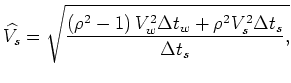where $V_w$ is water velocity, $V_s$ is the current estimate of sediment velocity, $\Delta t_w$ is two-way traveltime in the water layer, and $\Delta t_s$ is two-way traveltime in the sediments. At the first iteration $V_s$ is set to water velocity. I picked the values of the traveltime intervals from the section displayed in Figure 5 and set $\Delta t_w$=.018 s and $\Delta t_s$=.012 s. Entering these values and $\rho$=1.225 into equation 2 results into $\widehat{V_s}$=2.250 km/s.

This velocity is slightly higher than the final one because of the limitation of the linearized residual migration I used. For large velocity errors, this residual migration undercorrects the image because it does not take into account ray bending. The error encountered in this case is larger than 20%. Consequently, the residual-migration parameter $\rho$ is overestimated. However, another iteration of the velocity updating is sufficient to converge. My conjecture about the cause of the velocity-correction overshooting is supported by Figure 12, as discussed below.

The two panels in Figure 8 show respectively the result of the focusing analysis after migrating the data with the intermediate velocity function, $V_s$=2.250 km/s (panel a), and the final velocity function, $V_s$=2.155 km/s (panel b). This final velocity for the sediments was estimated using equation 2 with $\rho$=0.975; that is, the $\rho$ value that corresponds to the maximum in Figure 8a. The semblance peak in Figure 8b occurs at $\rho$=1, indicating that the process has converged. The estimated value of 2.155 km/s for the sediment velocity is consistent with the geologic information available from well drilled near the location where the data were acquired.

Sembl3-overn Figure 7. Image-focusing semblance computed from the initial migrated section and spatially averaged over the analysis window. Figure 6. [CR]

Sembl-iter12-overn Figure 8. Image-focusing semblance computed from: (a) the intermediate migrated section, and (b) the final migrated section. [CR]

Figure 9 summarizes the iterative velocity-estimation process by showing the velocities as a function of depth at each iteration. The solid line (labeled as ``Initial'') represents the starting velocity, constant and equal to water velocity. The dashed line (labeled as ``Intermediate'') represents the result of the first correction, which slightly overshoots. The dotted line (labeled as ``Final'') represents the final velocity function.

Figure 10 compares the images obtained with the three velocities in the analysis window. Figure 10a shows a zoom into the image shown in Figure 6. Figure 10b shows a zoom into the migrated image obtained using the overcorrected velocity function, and Figure 10c shows the final image. Compared with the other two images, the final image shows substantial improvement in the continuity of the reflectors and a reduction in the amount of crossing events.

Vel-overn Figure 9. Velocity functions used for the three iterations of velocity-estimation process. [ER]

Mig-win-overn
Figure 10. Migrated images in the analysis window for the three iterations: (a) initial velocity, (b) intermediate velocity, and (c) final velocity. [CR]

Figure 11 compares the entire image obtained with the initial velocity (top panel) with the entire image obtained with the final velocity (bottom panel). The improvement in the image are substantial also outside of the analysis window. The image for the dipping interface between the sediments and serpentinite at the left of the analysis window (between 60 and 90 meters along the midpoint axis) is more continuous in the final than in the initial image. The reflections just below this interface are also better focused in Figure 11b than in Figure 11a. Similarly, the reflector at the bottom of the sediment layer on the right of the analysis window (between 140 and 160 meters along the midpoint axis) is more continuous in the final image than in the initial one.

Finally, Figure 12 supports my previous conjecture that the overestimation of the velocity correction at the first iteration is caused by accuracy limitations of the linearized residual migration I employed when correcting for large velocity errors. This figure compares the analysis window for the final migrated image (top panel) with the analysis window taken from the residual migration of the first migrated image that corresponds to the picked value of $\rho$; that is, with $\rho=1.225$ (bottom panel). These two images are very similar, demonstrating that the first $\rho$ estimate is consistent with the final, and ``optimal'', velocity estimate. It leads to overshooting the interval-velocity correction because the residual migration is inaccurate. Notice that the differences in the vertical axis between the two sections are caused by the remapping to pseudo-depth of the residual-migrated section shown in Figure 12b.

Mig-overn
Figure 11. Comparison of the entire images obtained with: (a) initial velocity, and (b) final velocity. [CR]

ResMig-win-overn
Figure 12. Comparison of the migrated images in the analysis window for (a) final velocity, (b) residual migration of the starting image for $\rho$=1.225. The image-focusing method selected the bottom image to be the best focused image among the ensemble of residual migrated images obtained from the initial migration. [CR]

Measuring velocity from zero-offset data by image focusing analysis