Measuring velocity from zero-offset data by image focusing analysis

Image-focusing velocity estimation

In this section I briefly summarize the procedure I used to produce the results shown in the following two sections. The procedure is a simplification to zero-offset data of the method I presented in Biondi (2009).

The process starts from a partially-focused migrated image ${\bf R}\left({\bf x}\right)$, which is function of spatial coordinate vector ${\bf x}=\left\{z,x\right\}$, and continues with the following steps:

1. Perform residual migration on the initial image to produce an ensemble of residual-migrated images ${\bf R}\left({\bf x},\rho\right)$, where the parameter $\rho$ is the ratio between the new migration velocity and the migration velocity used for the initial migration.

2. Estimate the local apparent structural dips in the residual-migrated images.

3. Dip-decompose the residual-migrated images, ${\bf R}\left({\bf x},\rho\right)$, to obtain the dip-decomposed images ${\bf R}\left({\bf x},\alpha ,\rho\right)$, where $\alpha$ is the structural dip.

4. Perform the curvature correction (equation 2 in Biondi (2009)) of the dip-decomposed residual-migrated images, ${\bf R}\left({\bf x},\alpha ,\rho\right)$, using the local-dip information extracted at step 2. The results of this process are the curvature-corrected images ${\bf R}_{{\rm Curv}}\left({\bf x},\alpha ,\rho,{R}\right)$, where ${R}$ is the radius of curvature.

5. Compute image-focusing semblance as a function of $\rho$ and ${R}$ by applying the following equation,

   $$S_\alpha \left({\bf x},\rho,{R}\right)= \frac{ \left[\sum_\alpha ... ...ha } \sum_\alpha {\bf R}_{{\rm Curv}}\left({\bf x},\alpha ,\rho,{R}\right)^2 },$$ (1)

   
   
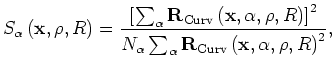
   where $N_{\alpha }$ is the number of dips included in the semblance computation.

6. Average the semblance computed using equation 1 over a spatial analysis window, after clipping out the smallest values of the semblance to remove noise and artifacts.

To perform the residual migration listed in step 1 of the procedure outlined above I used the linearized residual migration described in the Appendix of Biondi (2008). Other residual migration methods could be used, such as the one presented in Sava (2003). To simplify the analysis, I remapped the residual-migrated sections to pseudo-depth; that is, I remapped the depth axis of residual-migrated images according to the relationship $\tilde{z}=z/\rho$, where $\tilde{z}$ is pseudo-depth (Sava, 2004).

To estimate the local structural dips required by step 2, I used the Seplib program Sdip that implements a variant of the algorithms described by Fomel (2002). Any other local-dips estimator would be suitable. When performing the curvature correction at step 4, I define the curvature to be positive if the reflector frowns down (e.g. anticline) and negative if the reflector smiles up (e.g. syncline). The parameter $N_{\alpha }$ required for evaluating the focusing semblance at step 5 can be spatially varying according to the actual dip spectrum in the image. I kept it constant for my tests.

Measuring velocity from zero-offset data by image focusing analysis