Theory and practice of interpolation in the pyramid domain

acknowledgments

We thank Shuki Ronen and Xukai Shen for numerous discussion on this topic. We also thank the sponsors of the Stanford Exploration Project for their financial support.

comp-tx-fx-fu-synthplane3
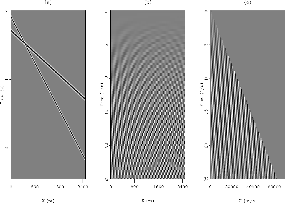
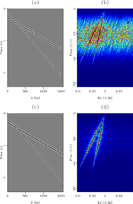
Figure 1. Two plane waves in (a) $(t,x)$, (b) $(\omega ,x)$ and (c), $(\omega ,u)$ domains.(b) and (c) show the real parts only. [NR]

comp-tx-fu-pyramid-60-synthplane2
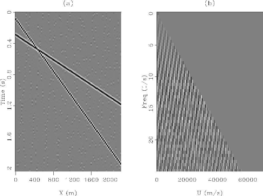
Figure 2. Illustration of transformation artifacts: (a) is ${\bf LL'd}$ back in the $(t,x)$ domain and (b) is the real part $\Re ({\bf L'd})$, where ${\bf d}$ is the data in Figure 1a. The slowest event, with the highest wavenumber component on the $u$ axis, disappears due to the parameterization of the pyramid transform. [NR]

comp-tx-fu-pyramid-5-synthplane2
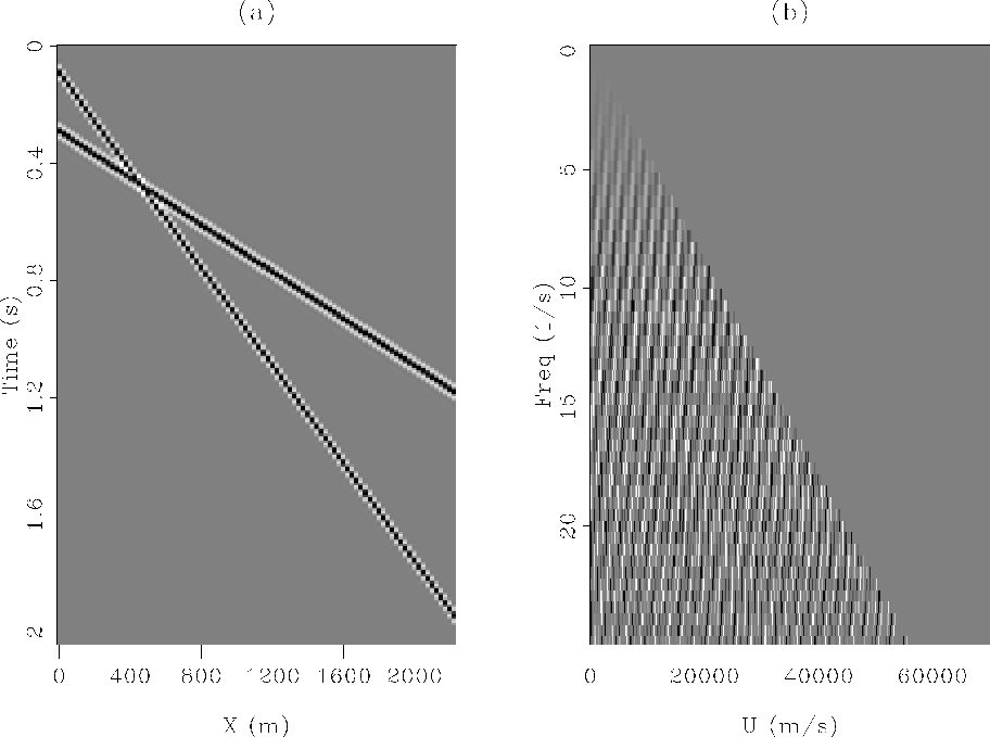
Figure 3. Same as Figure 2 but with a 12 times finer horizontal sampling on the $u$ axis. The two plane-waves are recovered. Some noise is still present due the linear interpolation operator. [NR]

comp-tx-fu-pyramid-5iter-synthplane2
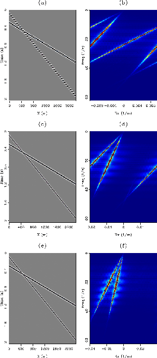
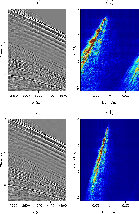
Figure 4. Illustration of the iterative process to attenuate the effects of linear interpolation. (a) is ${\bf L \tilde m}= {\bf L(L'L)^{-1}L'd}$ back in the $(t,x)$ domain and (b) is $\Re({\bf\tilde m})$. The noise in Figure 3a has been attenuated. [NR]

aliased-synthetic2
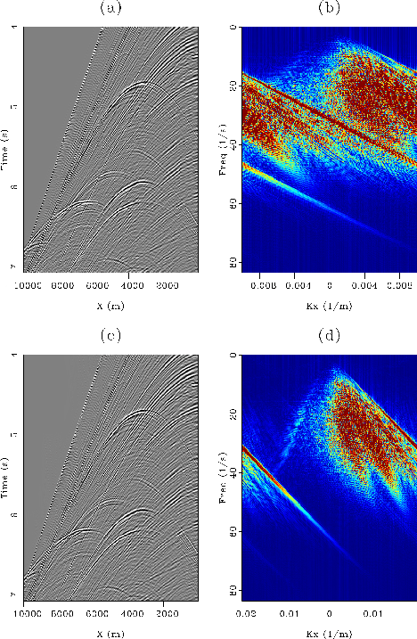
Figure 5. Interpolation results for aliased data: (a) Shows the input data at $\Delta x$=50 m and its corresponding $FK$ spectrum in (b). The slowest event is aliased for frequencies above 13 Hz and the fastest for frequencies above 22 Hz. (c) Shows the interpolation result with $\Delta x$=25 m and the corresponding $FK$ spectrum in (d). The slowest event is still aliased above 22 Hz. (e) Shows the interpolation result with $\Delta x$=12.5 m and the corresponding $FK$ spectrum in (e). The data in (a) have been dealiased for all frequencies. [NR]

aliased-bp
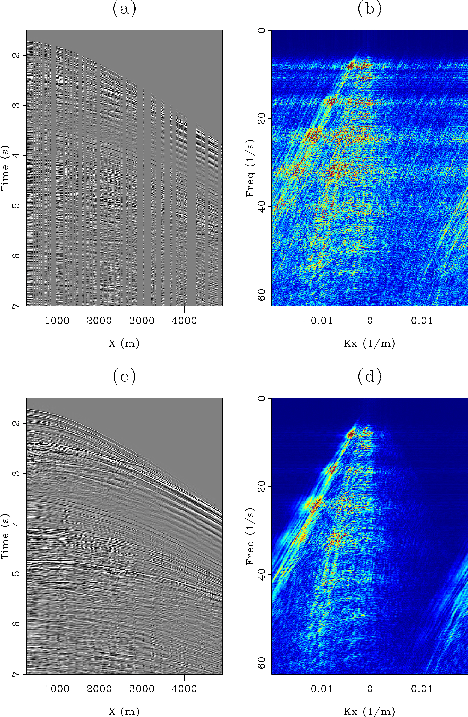
Figure 6. Interpolation results of a realistic synthetic data experiment. (a) Shows the input data on a 50 m grid with its $FK$ amplitude spectrum in (b). (c) Shows the same data after interpolation on a 25 m grid ($FK$ spectrum in (d)). All the events have been correctly interpolated but some aliasing remains. [NR]

aliased-gm
Figure 7. Interpolation results of a shot gather from the Gulf of Mexico. (a) Shows a close-up of the input data on a 26 m grid with its $FK$ amplitude spectrum in (b). (c) Shows the same data after interpolation on a 13 m grid ($FK$ spectrum in (d)). All the events have been correctly interpolated. [NR]

irregular-synth
Figure 8. Interpolation of irregularly-sampled data. (a) Shows the input data binned onto a regular grid before interpolation where 50$\%$ of the traces are missing and its corresponding $FK$ spectrum in (b). Interpolation results are shown in (c) ($FK$ spectrum in (d)): the linear events are recovered. [NR]

irregular-bp
Figure 9. Interpolation of a synthetic shot gather with irregular sampling. (a) Shows the input data binned onto a regular grid before interpolation and its corresponding $FK$ spectrum in (b). Interpolation results are shown in (c) ($FK$ spectrum in (d)). Our proposed algorithm recovers the missing traces where conflicting dips are present. [NR]

irregular-gm
Figure 10. Interpolation of a shot gather from the Gulf of Mexico with irregular sampling. (a) Shows the input data binned onto a regular grid before interpolation and its corresponding $FK$ spectrum in (b). Interpolation results are shown in (c) ($FK$ spectrum in (d)). The missing traces are reconstructed and there is no noticeable footprint left by the interpolation algorithm. [NR]

Theory and practice of interpolation in the pyramid domain