|
|
|
|
Least-squares migration/inversion of blended data |
Figure 13 shows the local Hessian operators for the blended acquisition geometries at different spatial locations in the subsurface. Note that the Hessian operators are far from unitary and contain many non-negligible off-diagonal elements, which contribute to the crosstalk in the migrated images.
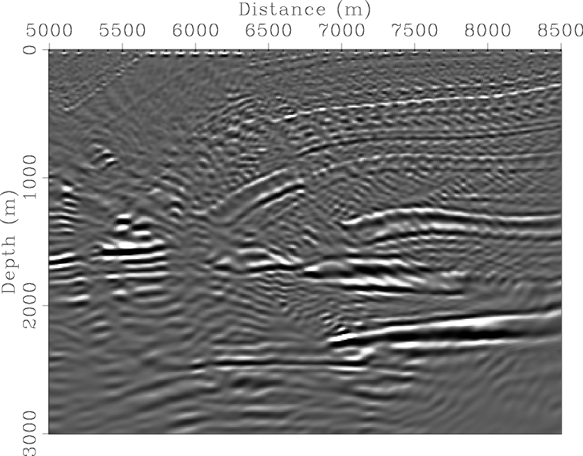
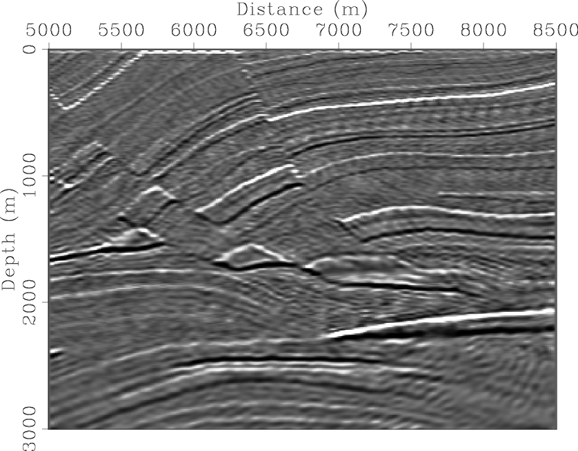
The migration and data-space LSI results are shown in Figure 14 and
Figure 15. In the inversion results,
a horizontal Laplacian operator that imposes horizontal continuities of the reflectivity is used
as the regularization operator ![]() .
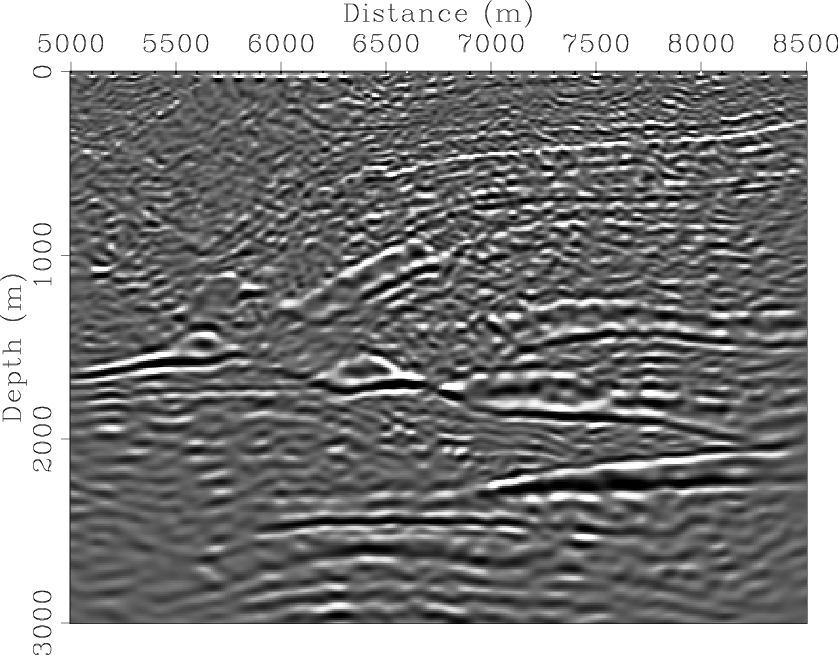
For both blended acquisition geometries, migration produces poor images
(Figure 14(a) and Figure 15(a)),
which are seriously contaminated by crosstalk artifacts.
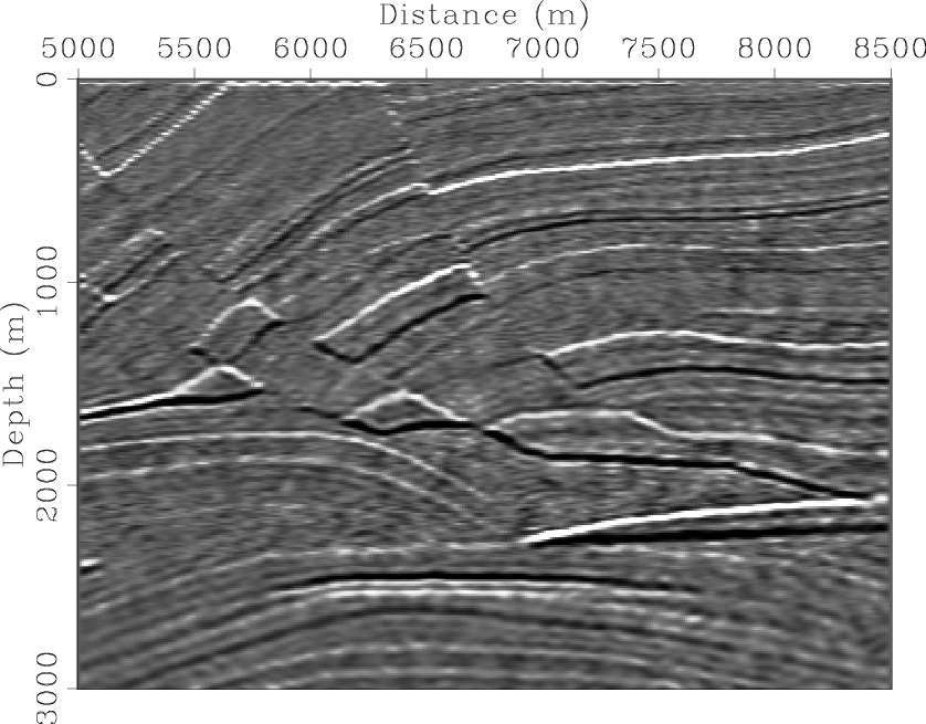
The data-space LSI, on the contrary, successfully removes
the crosstalk and we get good reconstruction of the reflectivity in the subsurface
(Figure 14(b) and Figure 15(b)).
.
For both blended acquisition geometries, migration produces poor images
(Figure 14(a) and Figure 15(a)),
which are seriously contaminated by crosstalk artifacts.
The data-space LSI, on the contrary, successfully removes
the crosstalk and we get good reconstruction of the reflectivity in the subsurface
(Figure 14(b) and Figure 15(b)).
|
|---|
|
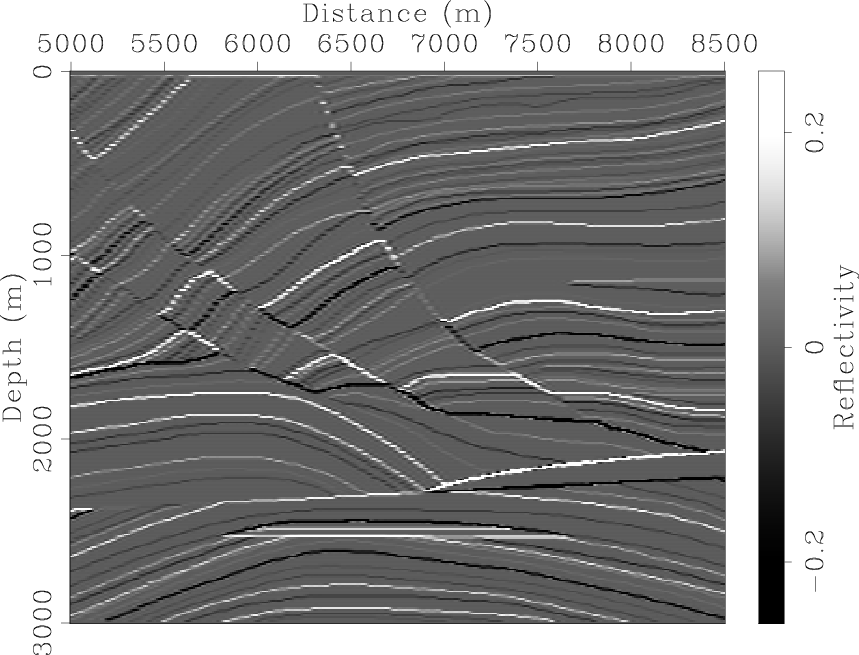
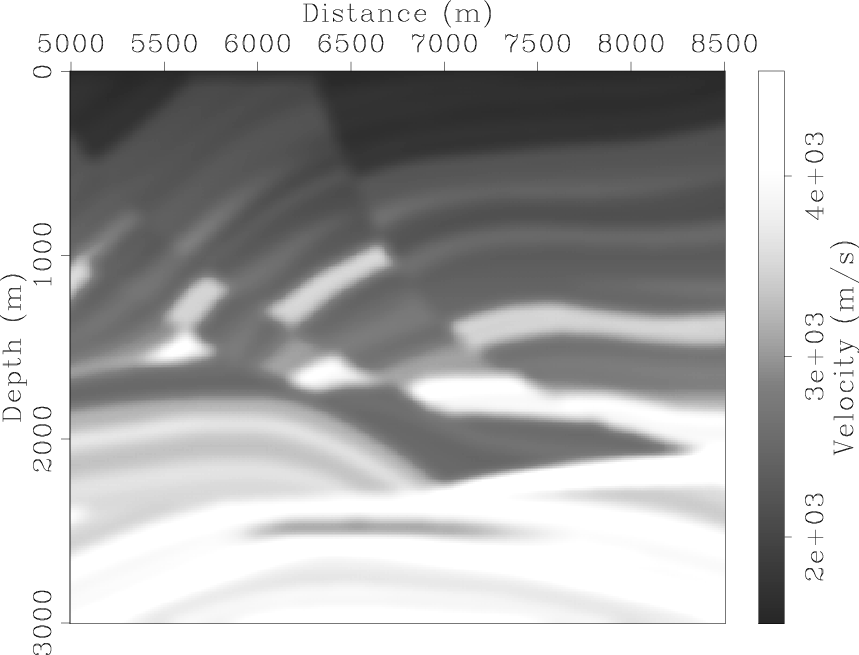
marm-refl,marm-vmod
Figure 11. The Marmousi model. (a) Reflectivity model; (b) background velocity model. [ER] |
|
|
|
|---|
|
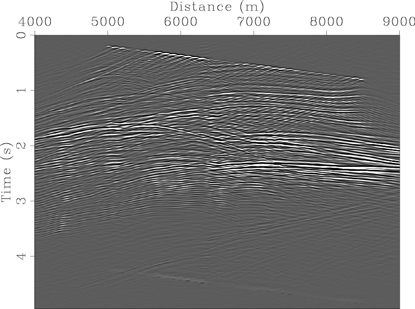
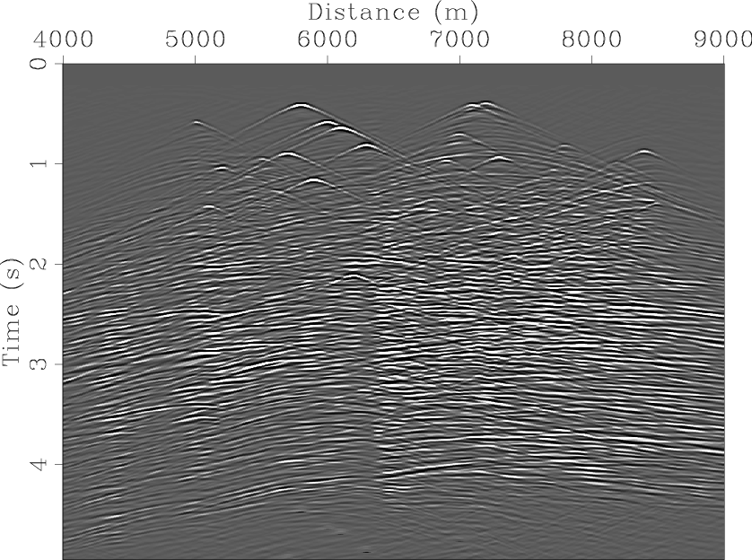
marm-trec-planes-2,marm-trec-randts
Figure 12. Synthesized blended shot gather for (a) linear-time-delay blended acquisition and (b) random-time-delay blended acquisition. [CR] |
|
|
|
|---|
|
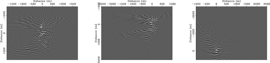
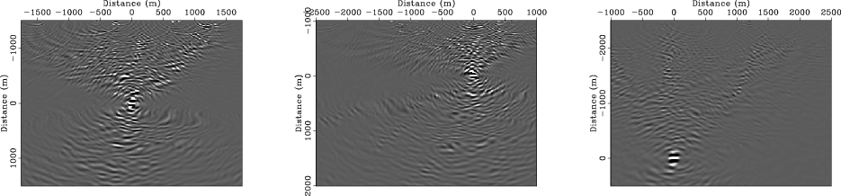
marm-hess-super-planes-2,marm-hess-super-randts
Figure 13. The local Hessian operators (rows of the full Hessian) at different locations for blended acquisition geometries. Panel (a) shows the results for linear-time-delay blending, while panel (b) shows the results for random-time-delay blending. In both (a) and (b), left, center and right panels are the local Hessians located at |
|
|
|
|---|
|
marm-imag-planes-2,marm-lsm-planes-2
Figure 14. Comparison between (a) migration and (b) data-space LSI for the linear-time-delay blended acquisition geometry. [CR] |
|
|
|
|---|
|
marm-imag-randts,marm-lsm-randts
Figure 15. Comparison between (a) migration and (b) data-space LSI for the random-time-delay blended acquisition geometry. [CR] |
|
|
|
|
|
|
Least-squares migration/inversion of blended data |