Kinematics in iterated correlations of a passive acoustic experiment

Stationary-phase analysis of conventional interferometry

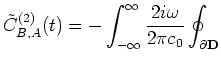
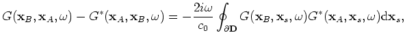
The phase of the correlation under the integral on the right-hand side of equation 2 changes rapidly as a function of source position. The dominant contribution to the integral comes from points at which the phase is stationary. Physically these positions correspond to source points from where the ray paths to both stations align. To analyze the stationary phases in the presence of a scatterer, we consider a homogeneous medium and study the time-domain expression of equation 2 using the first three terms in $C^{(2)}_{B,A}$ of equation 4:

$$G(\mathbf{x}_B,\mathbf{x}_A,t) - G(\mathbf{x}_A,\mathbf{x}_B,-t) =$$ (7)

$$\tilde{C}^{(2)}_{B,A}(t) = -\int_{-\infty}^{\infty}\frac{2i\omega}{2\pi c_0}\oint_{\partial \mathbf{D}} a_0(\mathbf{x}_B,\mathbf{x}_s,\omega)a_0^*(\mathbf{x}_A,\mathbf{x}_s,\omega) \mathrm{exp} \left\{ i\Omega_1 \right\} + \notag$$ (8)

$$a_0(\mathbf{x}_B,\mathbf{x}_s,\omega)a_1^*(\mathbf{x}_A,\mathbf{x}_s,\omega) \mathrm{exp} \left\{ i\Omega_2 \right\} + \notag$$ (9)

$$a_1(\mathbf{x}_B,\mathbf{x}_s,\omega)a_0^*(\mathbf{x}_A,\mathbf{x}_s,\omega) \mathrm{exp} \left\{ i\Omega_3 \right\} \mathrm{d}\mathbf{x}_s \mathrm{d}\omega, \notag$$ (10)

where $a_0$ and $a_1$ are amplitude factors. The rapid phases, $\Omega_1=\Omega_1(\mathbf{x}_s,\mathbf{x}_A,\mathbf{x}_B,\omega)$, $\Omega_2(\mathbf{x}_s,\mathbf{x}_A,\mathbf{x}_B,\omega)$ and $\Omega_3(\mathbf{x}_s,\mathbf{x}_A,\mathbf{x}_B,\omega)$, of the three terms are found using equations A-6 and A-11:

$$\Omega_1 = \omega \left[ t - c_0^{-1} \left\{ \vert\mathbf{x}_B - \mathbf{x}_s\vert - \vert\mathbf{x}_A - \mathbf{x}_s\vert \right\} \right],$$ (11)

$$\Omega_2 = \omega \left[ t - c_0^{-1} \left\{ \vert\mathbf{x}_B - \mathbf{x}... ...A - \mathbf{x}_c\vert - \vert\mathbf{x}_c - \mathbf{x}_s\vert \right\} \right],$$ (12)

$$\Omega_3 = \omega \left[ t - c_0^{-1} \left\{ \vert\mathbf{x}_B - \mathbf{x}... ...c - \mathbf{x}_s\vert - \vert\mathbf{x}_A - \mathbf{x}_s\vert \right\} \right],$$ (13)

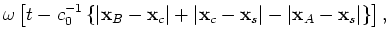where $\mathbf{x}_c$ is the position of the scatterer.

We analyze these rapid phases using the stationary-phase method, keeping $\mathbf{x}_A$ and $\mathbf{x}_B$ fixed and varying $\mathbf{x}_s$. According to the stationary-phase method, the dominant contribution comes from stationary phases where

$$\partial_\omega \Omega=0 \hspace{.5cm} \mathrm{and} \hspace{.5cm} \nabla_{\mathbf{x}_s} \Omega = \mathbf{0}.$$ (14)

From the rapid phase, 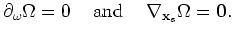$\Omega_1$, of the first term in equation 6, we find stationary points for which

$$t = c_0^{-1} \left\{ \vert\mathbf{x}_B - \mathbf{x}_s\vert - \ver... ...mathbf{x}_s\vert = \nabla_{\mathbf{x}_s} \vert\mathbf{x}_A - \mathbf{x}_s\vert.$$ (15)

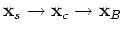
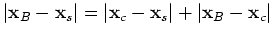
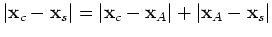
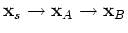
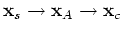
The second condition requires the points $\mathbf{x}_A$ and $\mathbf{x}_B$ to be aligned along a line issuing from $\mathbf{x_s}$. When the stations and source are aligned as $\mathbf{x}_s \rightarrow \mathbf{x}_A \rightarrow \mathbf{x}_B$, the first condition gives $t = c_0^{-1} \left\{ \vert\mathbf{x}_B - \mathbf{x}_A\vert \right\}$. When the stations and source are aligned as $\mathbf{x}_s \rightarrow \mathbf{x}_B \rightarrow \mathbf{x}_A$, the first condition gives $t = - c_0^{-1} \left\{ \vert\mathbf{x}_B - \mathbf{x}_A\vert \right\}$.

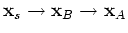From rapid phase 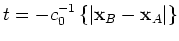$\Omega_2$ of the second terms in equation 6, we find stationary points for which

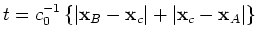
$$t= c_0^{-1} \left\{ \vert\mathbf{x}_B - \mathbf{x}_s\vert - \vert... ...mathbf{x}_s\vert = \nabla_{\mathbf{x}_s} \vert\mathbf{x}_c - \mathbf{x}_s\vert.$$ (16)

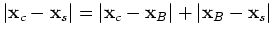
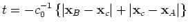
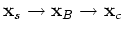The second condition requires the points $\mathbf{x}_B$ and $\mathbf{x}_c$ to be on a line issuing from $\mathbf{x}_s$. When station B, as well as the scatterer and sources are aligned as $\mathbf{x}_s \rightarrow \mathbf{x}_B \rightarrow \mathbf{x}_c$, then $\vert\mathbf{x}_c - \mathbf{x}_s\vert = \vert\mathbf{x}_c-\mathbf{x}_B\vert + \vert\mathbf{x}_B-\mathbf{x}_s\vert$, and the first condition states that $t =- c_0^{-1} \left\{ \vert\mathbf{x}_B - \mathbf{x}_c\vert + \vert\mathbf{x}_c - \mathbf{x}_A\vert \right\}$. When station B, the scatterer and the source are aligned as $\mathbf{x}_s \rightarrow \mathbf{x}_c \rightarrow \mathbf{x}_B$, then $\vert\mathbf{x}_B - \mathbf{x}_s\vert = \vert\mathbf{x}_c-\mathbf{x}_s\vert + \vert\mathbf{x}_B-\mathbf{x}_c\vert$, and the first condition states that $t = c_0^{-1} \left\{ \vert\mathbf{x}_B - \mathbf{x}_c\vert - \vert\mathbf{x}_A - \mathbf{x}_c\vert \right\}$.

From rapid phase 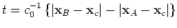$\Omega_3$ of the second terms in equation 6, we find stationary points for which

$$t = c_0^{-1} \left\{ \vert\mathbf{x}_B - \mathbf{x}_c\vert + \ver... ...mathbf{x}_s\vert = \nabla_{\mathbf{x}_s} \vert\mathbf{x}_c - \mathbf{x}_s\vert.$$ (17)

The second condition requires the points $\mathbf{x}_A$ and $\mathbf{x}_c$ to be on a line issuing from $\mathbf{x}_s$. When station A, as well as the scatterer and sources are aligned as $\mathbf{x}_s \rightarrow \mathbf{x}_A \rightarrow \mathbf{x}_c$, then $\vert\mathbf{x}_c - \mathbf{x}_s\vert = \vert\mathbf{x}_c-\mathbf{x}_A\vert + \vert\mathbf{x}_A-\mathbf{x}_s\vert$, and the first condition states that $t = c_0^{-1} \left\{ \vert\mathbf{x}_B - \mathbf{x}_c\vert + \vert\mathbf{x}_c - \mathbf{x}_A\vert \right\}$. 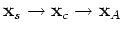When station A, the scatterer and sources are aligned as $\mathbf{x}_s \rightarrow \mathbf{x}_c \rightarrow \mathbf{x}_A$, then $\vert\mathbf{x}_A - \mathbf{x}_s\vert = \vert\mathbf{x}_A-\mathbf{x}_c\vert + \vert\mathbf{x}_c-\mathbf{x}_s\vert$, and the first condition states that $t = c_0^{-1} \left\{ \vert\mathbf{x}_B - \mathbf{x}_c\vert - \vert\mathbf{x}_A - \mathbf{x}_c\vert \right\}$. 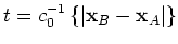For a more extensive treatment of stationary-phase positions in conventional interferometry, see Schuster et al. (2004); Snieder et al. (2006); Snieder (2004) and Garnier and Papanicolaou (2009).

Kinematics in iterated correlations of a passive acoustic experiment