Kinematics in iterated correlations of a passive acoustic experiment

Conventional versus iterative interferometry

Conventional seismic interferometry (SI) retrieves the Green's function between two stations by correlating, $C^{(2)}$, records of an ambient field, in which the energy is equipartitioned, recorded at both stations. It is generally assumed that energy equipartitioning should be obtained after averaging over sources that excite the background field (Snieder et al., 2007). Sources located at stationary phases are necessary to retrieve high-quality EGFs. For example, the stationary-phase region of the Green's function between stations $A$ and $B$ in Figure 1(a) is located on a ray path from station $B$ extending to and beyond station $A$ [gray shading on left side of Figure 1(a)]. Correlating responses from these sources recorded at $A$ and $B$ will retrieve a high-quality EGF. However, because the sources in Figure 5(b) are not located in the stationary-phase region, correlating responses from these sources recorded at $A$ and $B$ will retrieve a low-quality EGF.

mainC2drawnew1,mainC2drawnew2
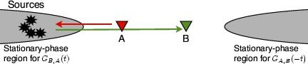
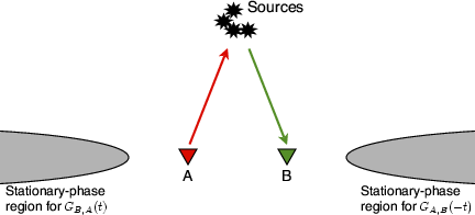
Figure 1. Source positions for respectively (a) high-quality and (b) poor quality Green's function estimation by conventional SI. Stationary-phase regions are indicated by gray areas. $\mathbf{[NR]}$

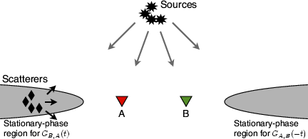
Some proposed methods to compensate for anisotropic illuminations include: (a) Beam forming and weighting (Stork and Cole, 2007) or $\tau-p$ filtering (Ruigrok et al., 2008) the data for different directionality components. (b) Estimating a radiation pattern by autocorrelating the down-going wave field and correcting by deconvolution (van der Neut et al., 2008; van der Neut and Bakulin, 2008). (c) Multidimensional deconvolution after the identification of individual responses (Wapenaar et al., 2008). Finally (d), Stehly et al. (2008) propose a novel procedure to improve EGFs by using scatterers positioned at the stationary-phase positions that act as secondary Huygens' sources, as illustrated in Figure 2. Their method requires three steps: First, the recordings at two main stations are correlated with a network of auxiliary stations. Each correlation yields an EGF. Second, each EGF is muted for times prior to an estimated arrival time. Third, a correlation, $C^3$, is evaluated between the muted EGF pairs estimated for each auxiliary station. That correlation is subsequently averaged across the network of auxiliary stations.

mainC4drawnew0 Figure 2. Illustration of how scatterers acting as secondary Huygens' sources can illuminate stations $A$ and $B$ from a stationary-phase region, while the primary sources are located outside the stationary-phase regions. $\mathbf{[NR]}$

Kinematics in iterated correlations of a passive acoustic experiment