Delayed-shot migration in TEC coordinates

3D Wide-azimuth synthetic tests

This section presents the inline delayed-shot migration algorithm test results on a wide-azimuth synthetic data set generated from a realistic 3D Gulf of Mexico velocity model. Figure 5 presents some depth slices and sections through the model. The velocity model is comprised of typical Gulf of Mexico sedimentary profile with a velocity gradient of approximately $0.2$ s$^{-1}$, with a number of salt bodies of complex 3D geometry characterized by smoothly varying salt tops and steep flanks below overhangs. Key imaging targets include the steep salt flanks and the on-lapping sedimentary units that comprise the likely exploration areas.

VELCUT
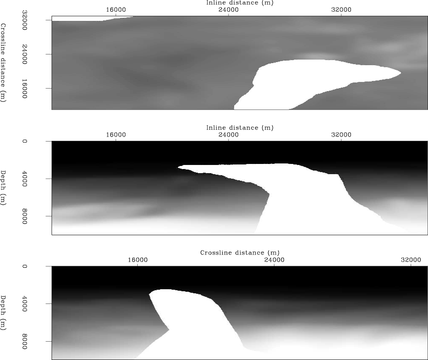
Figure 5. Depth section and inline crossline sections of the Gulf of Mexico velocity model through complex 3D salt bodies. Top: 3900 m depth slice. Middle: 33000 m inline section. Top: 16000 m crossline section. ER

Table 2 summarizes the acquisition geometry of the data set. The data used for migration consisted of 72 sail lines separated 250 m apart. Each sail line consists of 100 shots sampled at a 250 m shot interval. The receiver pattern for each shot record contains 321 inline samples with a maximum offset of $\pm$8000 m computed at a 50 m interval, and 161 crossline samples with a maximum offset of $\pm$4000 m at a 50 m interval.

Table 2: Parameters associated with the 3D synthetic data set.

Source Parameter	Value	Receiver Parameter	Value
Number of sail lines	72	Max. inline offset (m)	$\pm$8000
Sail line interval (m)	250	Max. crossline offset (m)	$\pm$4000
Shots per sail line	100	Inline receiver interval (m)	50
Shot interval (m)	250	Crossline receiver interval (m)	50

A total of 192 frequencies were selected for migration starting at 1.42 Hz at a sampling rate of 0.075 Hz. Filtered data from each sail line data were transformed into a plane-wave data set by phase-encoding over a range of inline ray parameters, $p_{\xi_1}$. I selected a total of 101 inline ray parameters between $\pm$8.33x10$^{-4}$ sm$^{-1}$ at a sampling rate of 8.33x10$^{-6}$ sm$^{-1}$. Given the $1500$ ms$^{-1}$ water velocities at the surface, the maximum values correspond to a surface take-off angle of $\pm 38.7^\circ$.

I applied the inline delayed-shot migration technique to the plane-wave data on a sail-line by sail-line basis, which allowed for a coarse-grain computational parallelism at a scripting level. (The migration code was also OMP-enabled, which led to a second level of coarse-grain parallelism over the frequency axis.) Migration runs were conducted for Cartesian coordinate (CC) and TEC geometries with both tilting and non-tilting meshes. For CC migrations, the data volumes were zero-padded with 40 samples on each inline side and 95 samples on each crossline side. The data volume for TEC migrations were padded with 40 samples on the inline sides, but only one sample on each crossline side because the coordinate system aperture expands naturally in the crossline direction.

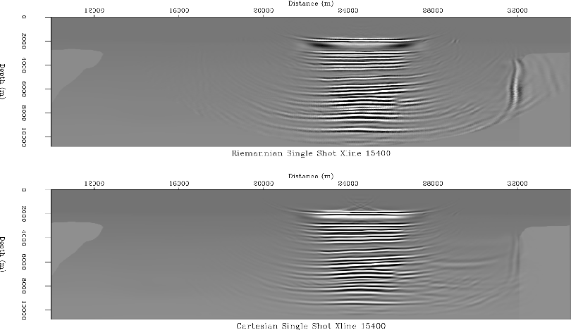
Figure 6 presents the 15400 m cross section from the 24500 m sail-line migration image (for 101 plane-waves) for the TEC (top panel) and the CC (bottom panel) geometries. The gently dipping sedimentary reflections in both sections are imaged across a 6000 m swath. The TEC migration, relative to that in CC geometry, shows a significant improvement in the vertical salt flank on the right-hand-side of the image. Although the salt-flank is weakly present in the CC image under strong clipping, it is mis-positioned due to the $80^\circ$ limit of extrapolation operator accuracy.

TESTY15400
Figure 6. Sections for the 24500 m sail line at the 15400m crossline coordinate. Top: Elliptical-cylindrical coordinate image. Bottom: Cartesian coordinate image. NR

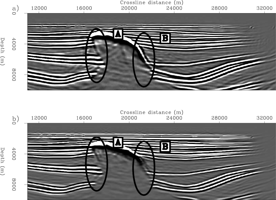
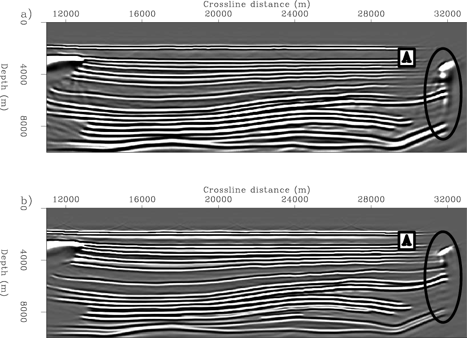
Figures 7 and 8 present crossline sections from the full TEC and CC image volumes. Figure 7 presents the EC and Cartesian crossline sections at the 33700 m inline coordinate in the upper and lower panels, respectively. The TEC image has an improved left-hand salt flank (marked A) that is more correctly positioned relative to the CC image. Similarly, the right-hand salt flank (marked B) is more accurately positioned and forms a more continuous reflector.

FIG3
Figure 7. crossline sections through the velocity model and full image volumes at inline coordinate 33700 m. Top panel: Elliptical-cylindrical coordinate image. Bottom panel: Cartesian coordinate image. The imaging improvements for the left-hand salt flank are denoted by the oval marked A. The oval marked B illustrates a more continuous and correctly placed reflector in the TEC coordinate system. NR

Figure 8 presents the 15100 m crossline sections extracted from the two image volumes. Note the differences in the vertical right-hand salt flank (marked A) between the ECC (top panel) and CC (bottom panel) images. The TEC image exhibits a stronger reflector that is better positioned than that in the CC image (again because of the high-angle limits of the extrapolation operator).

FIG4
Figure 8. crossline sections through the velocity model and full image volumes at inline coordinate 15100 m. Top panel: Elliptical-cylindrical coordinate image. Bottom panel: Cartesian coordinate image. The oval marked A indicates the location of the vertical salt flank that is better imaged in TEC coordinates. NR

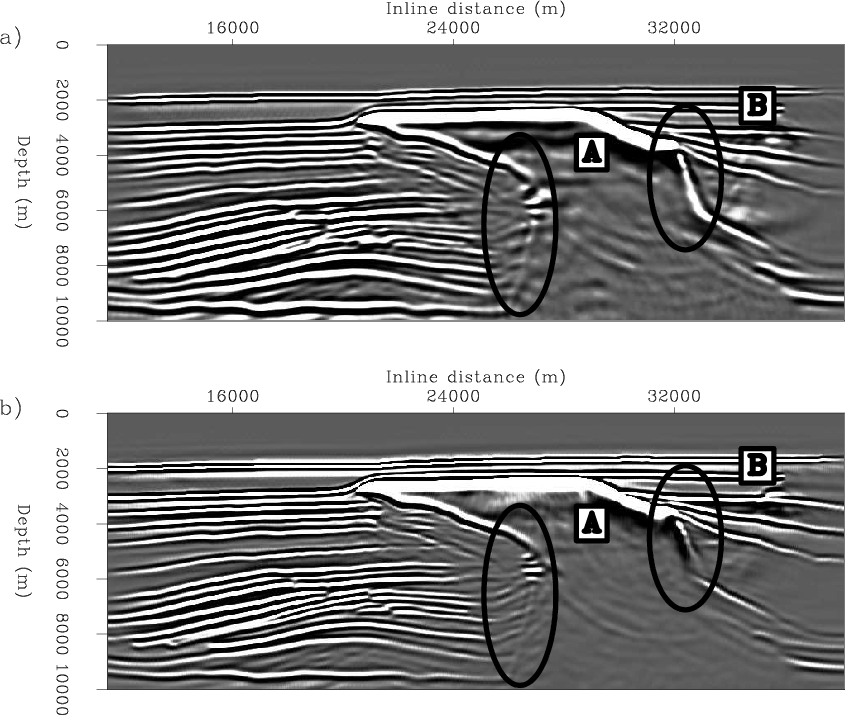
Figure 9 shows the 21750 m inline section through the complete TEC (upper panel) and CC (lower panel) image volumes. The left-hand salt flank (marked A) is more accurately located and continuous in the TEC image. The right-hand salt flank (marked B), again, is more continuous in the TEC image. Another observation is that the TEC image (and in Figures 7-8) does not contain the same spatial frequency content as the CC images (see below).

FIG1
Figure 9. Inline sections through the velocity model and full image volumes at crossline coordinate 21750 m. Top panel: Velocity section. Middle panel: Elliptical-cylindrical coordinate image. Bottom panel: Cartesian coordinate image. The left-hand salt flank, shown in oval A, is more accurately positioned in the TEC coordinate image, while the right-hand flank, marked by oval B, is similarly more accurately positioned and continuous. NR

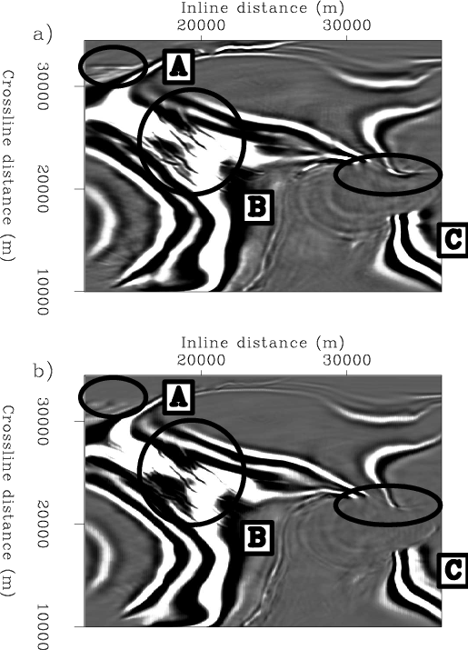
Figure 10 presents slices extracted at 6150 m depth from the TEC (top panel) and CC (bottom panel) images. The images are again fairly similar, though are there slight differences that correspond to amplitude differences between the weakly imaged steep flank reflectors. Examples include the regions marked A and C that corresponds to the salt flanks in Figure 9 and Figure 7, respectively. Finally, the migration algorithm has well-imaged the set of channels denoted in region B in both coordinate system images.

FIG5
Figure 10. Depth slices through the velocity model and image volumes at 6150 m depth. Top panel: Elliptical-cylindrical coordinate image. Bottom panel: Cartesian coordinate image. Oval A illustrates the improved TEC image for the vertical salt flank shown in Figure 8. Oval B demarcates a region where some of the smaller-scale fractures are well imaged in both images. Oval C shows the region where the near-vertical flank shown in TEC coordinate image in Figure 7 is better imaged. NR

Delayed-shot migration in TEC coordinates