|
|
|
|
Wave-equation tomography using image-space phase-encoded data |
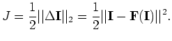
Under ![]() norm, the tomography objective function can be written as follows:
norm, the tomography objective function can be written as follows:
| (3) |
 with respect to the slowness
 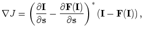 denotes the adjoint.
The linear operator
![]() , which defines a linear mapping from the slowness perturbation
, which defines a linear mapping from the slowness perturbation
![]() to the image perturbation
to the image perturbation
![]() , can be computed by expanding the image
, can be computed by expanding the image ![]() around the background slowness
around the background slowness
![]() . Keeping only the zeroth and first order terms, we get the linear operator
. Keeping only the zeroth and first order terms, we get the linear operator
![]() as follows:
as follows:
| (5) |
 ,
,
In the shot-profile domain, both source and receiver wavefields are downward continued with the one-way wave equations (Claerbout, 1971)
 is the source wavefield for a single frequency
  defines the point source function at is the source wavefield for a single frequency
  is the subsurface half-offset.
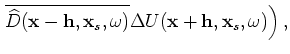
The perturbed image can be derived by the application of the chain rule to Equation 9:
 and
and
To evaluate the adjoint of the tomographic operator,
![]() , we first apply the adjoint of the imaging condition to get the perturbed source and receiver wavefields,
, we first apply the adjoint of the imaging condition to get the perturbed source and receiver wavefields,
![]() and
and
![]() , as follows
, as follows
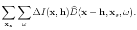
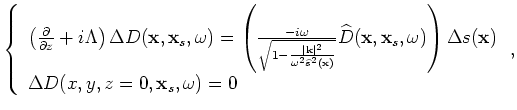
The perturbed source and receiver wavefields satisfy the following one-way wave equations, linearized with respect to slowness:
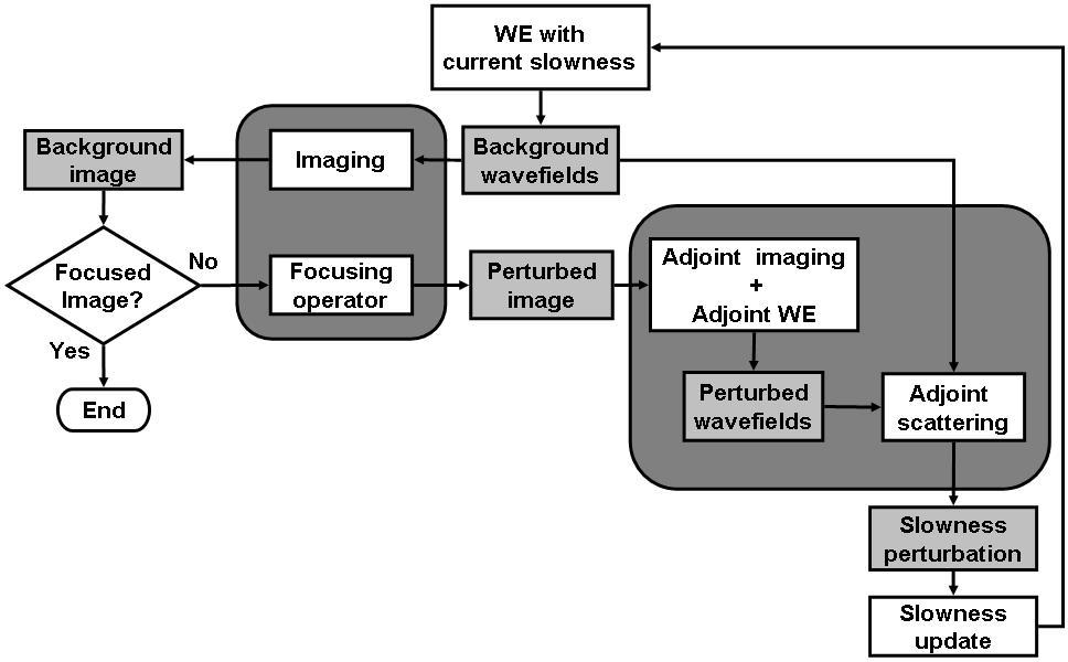
When solving the optimization problem, the gradient of the objective function is obtained by computing the perturbed wavefields using the adjoint of the imaging operator (equation 11), where the image perturbation results from the application of a focusing operator (equation 1) on the background image; then the scattered wavefields are obtained by applying the adjoint of the one-way wave equations 12 and 13; and, finally, the adjoint scattering operator cross-correlates the upward propagated the scattered wavefields with the modified background wavefields (term in the parenthesis on the right-hand side of equations 12 and 13). Figure 1 displays the image-space wave-equation tomography flowchart. The gray box on the left represents the process of obtaining the image perturbation, while the gray box on the right corresponds to the application of the adjoint of the wave-equation tomography operator. WE stands for wavefield extrapolation. The light gray boxes contain the wavefields, images and slowness perturbation. The processes and operators are represented as white boxes. More detailed information on how to evaluate the forward and adjoint operators can be found in Tang et al. (2008).
|
|---|
|
ISWET
Figure 1. Image-space wave-equation tomography flowchart. The gray box on the left represents the process of obtaining the image perturbation, while the gray box on the right corresponds to the application of the adjoint of the wave-equation tomography operator.[NR] |
|
|
|
|
|
|
Wave-equation tomography using image-space phase-encoded data |