Modeling, migration, and inversion in the generalized source and receiver domain

encoded sources and receivers

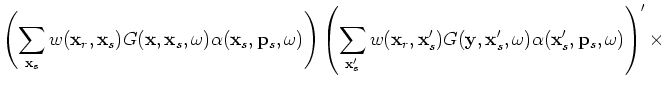
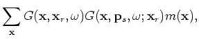
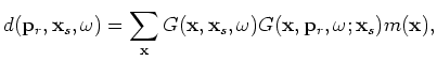
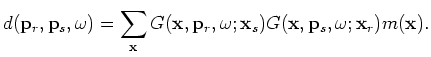
We can simultaneously encode the sources and the receivers as follows:

$$d({\bf p}_r,{\bf p}_s,\omega) = \sum_{{\bf x}_r} \sum_{{\bf x}_s}... ...s,\omega) \alpha({\bf x}_s,{\bf p}_s,\omega) \beta({\bf x}_r,{\bf p}_r,\omega),$$ (A-28)

where $\alpha({\bf x}_s,{\bf p}_s,\omega)$ and $\beta({\bf x}_r,{\bf p}_r,\omega)$ are defined by Equations 9 and 18, respectively, for plane-wave phase encoding, and by Equations 10 and 19, respectively, for random phase encoding.

Substituting Equations 1 into 28, notice that $w^2({\bf x}_r,{\bf x}_s)=w({\bf x}_r,{\bf x}_s)$. With the definition of $G({\bf x},{\bf p}_s,\omega;{\bf x}_r)$ and $G({\bf x},{\bf p}_r,\omega;{\bf x}_s)$ by Equations 12 and 21, we obtain the forward modeling equation in the encoded source and receiver domain:

$$d({\bf p}_r,{\bf p}_s,\omega) = \sum_{\bf x} G({\bf x},{\bf p}_r,{\omega};{\bf x}_s) G({\bf x},{\bf p}_s,{\omega};{\bf x}_r) m({\bf x}).$$ (A-29)

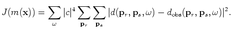
Now we minimize the following objective function in the encoded source and receiver domain (see Appendix C for derivation):

$$J(m({\bf x})) = \sum_{\omega}\vert c\vert^4\sum_{{\bf p}_r} \sum_... ...t d({\bf p}_r,{\bf p}_s,\omega)-d_{\rm obs}({\bf p}_r,{\bf p}_s,\omega)\vert^2.$$ (A-30)

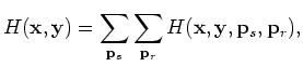
The gradient of the objective function in Equation 30 gives the following migration formula in the encoded source and receiver domain:

$$\nabla J({\bf x}) = \Re \left( \sum_{\omega}\vert c\vert^4\sum_{{... ...} G'({\bf x},{\bf p}_s,\omega;{\bf x}_r) r({\bf p}_r,{\bf p}_s,\omega) \right),$$ (A-31)

where 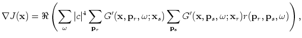$r({\bf p}_r,{\bf p}_s,\omega)$ is the residual in the encoded source and receiver domain:

$$r({\bf p}_r,{\bf p}_s,\omega) = d({\bf p}_r,{\bf p}_s,\omega)-d_{\rm obs}({\bf p}_r,{\bf p}_s,\omega).$$ (A-32)

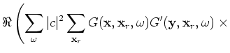
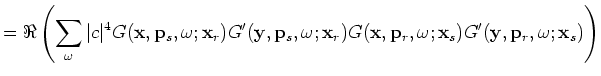
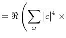
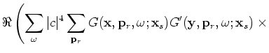
The Hessian is obtained as follows:

$$H({\bf x},{\bf y}) = \Re \left( \sum_{\omega}\vert c\vert^4 \sum_{{\bf p}_r} G({\bf x},{\bf p}_r,\omega;{\bf x}_s) G'({\bf y},{\bf p}_r,\omega;{\bf x}_s) \right. \times$$

$$\left. \sum_{{\bf p}_s} G ({\bf x},{\bf p}_s,\omega;{\bf x}_r) G'({\bf y},{\bf p}_s,\omega;{\bf x}_r) \right).$$ (A-33)

We can also rewrite Equation 33 as follows:

$$H({\bf x},{\bf y}) = \sum_{{\bf p}_s}\sum_{{\bf p}_r} H({\bf x},{\bf y},{\bf p}_s,{\bf p}_r),$$ (A-34)

where

$$H({\bf x},{\bf y},{\bf p}_s,{\bf p}_r)$$

$$= \Re \left( \sum_{\omega}\vert c\vert^4 G({\bf x},{\bf p}_s,\ome... ...f x},{\bf p}_r,\omega;{\bf x}_s) G'({\bf y},{\bf p}_r,\omega;{\bf x}_s) \right)$$

$$= \Re \left( \sum_{\omega}\vert c\vert^4 \right. \times$$

$$\left(\sum_{{\bf x}_s} w({\bf x}_r,{\bf x}_s) G({\bf x},{\bf x}_s... ...({\bf y},{\bf x}'_s,\omega) \alpha({\bf x}'_s,{\bf p}_s,\omega) \right)' \times$$

$$\left. \left(\sum_{{\bf x}_r} w({\bf x}_r,{\bf x}_s)G ({\bf x},{\... ...({\bf y},{\bf x}'_r,\omega)\beta({\bf x}'_r,{\bf p}_r,\omega) \right)' \right).$$ (A-35)

Equation 35 is equivalent to Equations 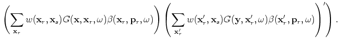$17$ and C-$1$ in Tang (2008), which are called the simultaneously encoded Hessian. However, Equation 35 is more general, because it is not limited to OBC or land acquisition geometry. Up to this point, we have proved that both the simultaneously encoded Hessian and the Hessian in the encoded source and receiver domain are derived from the same forward modeling equation defined in 29.

Modeling, migration, and inversion in the generalized source and receiver domain