Next: PEF estimation and Missing
Up: Methodology
Previous: Methodology
I discussed the 2D pyramid transform in Shen (2008), and the 3D version is almost the same, except that some scalars become vectors. In the 3D pyramid transform, spatial grid spacing is calculated for each frequency  using the equation
 |
(1) |
where
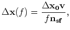 ,
,
 ,
,  and
and
 are all 2D vectors.
 is the uniform spatial grid spacing in the original -
 data, is the velocity that controls the slope of the pyramid and
 is the sampling factor in pyramid domain. By changing this factor we can control how densely the pyramid domain is sampled. In situations where events to be interpolated are not perfectly stationary, dense sampling is preferrable since the information in the low frequencies cannot be represented well by only a few points. In 3D, the inversion scheme that transforms data in - space to the pyramid domain is as follows:
 |
(2) |
where 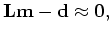 is the data in the pyramid domain,
  is the known data in - space, and
  is the 2D linear interpolation operator in 3D pyramid transform. The 3D pyramid transform from pyramid domain to - domina uses the following equation :
 |
(3) |
Where now  is known and
  is unknown data in - space.
Next: PEF estimation and Missing
Up: Methodology
Previous: Methodology
2009-04-13